Creating spiral oriented sub volume»
This guide explains how to create spiral based boxes.
The boxes can be used as ROIs for further analysis (Compartmentalization, gradient distribution, heat map, etcetera)

See also
Opening the working dataset
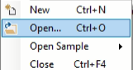
- Select Open... from the file menu.
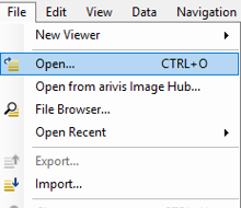
- Select the dataset from the file browser.
The dataset is a multi dimensional, discrete, representation of your real sample volume. It can be structured as a Z series of planes (Optical sectioning) of multiple channels (dyes) in a temporal sequence of time points (located in several spatial positions).
Usually, the dataset shows a single experimental situation (a complete experiment can be composed by several datasets). The datasets are available as graphic files saved in plenty of file formats (standard formats as well as proprietary formats).
Note: The dataset is visualized according to the current rendering setting parameters. Refer to the arivis Pro Help for more details.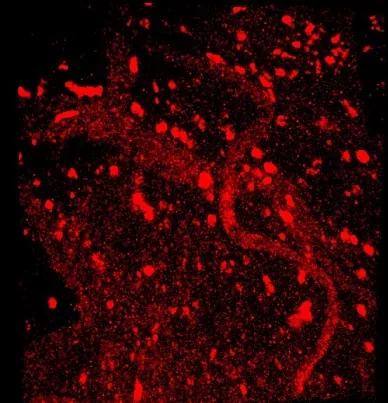
Drawing the reference 3D polyline
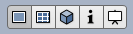
- Switch the Viewing area from 4D to 2D view mode.
- Select the Place a new object tool.
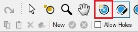
- Select the 3D Polyline tool.

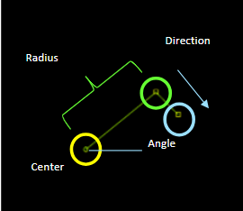
- Draw the 3D Polyline over any Z plane. The 1st point represents the center of the spiral, while the 2nd point defines the radius and the starting angle.
The 3rd defines the direction according to the following schema: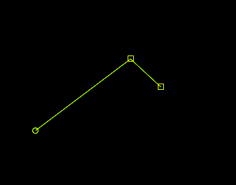
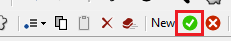
- Press the green icon to confirm the 3D Polyline.
- The TAG Manual is now available in the data table.
Loading the Python script
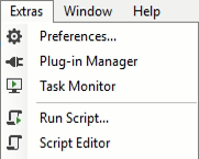
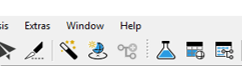
- Open Python Script Editor. From the Extra menu, select Script Editor.
- Load the Free-Oriented Sub-volume Python Script.
- Browse the folder on which the file has been saved.
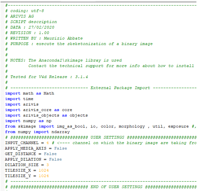
Only the parameters located in the USER SETTING area can be modified. Don’t change any other number, definition or text in the code outside this dedicated area.
Setting the script features
- In order to define the spiral distributed sub-regions (sampling volume) features, some parameters of the script should be adjusted to match your analysis needs. These parameters are located in the code area labeled as
USER SETTING.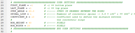
- Set the Z planes range.
FIRST_PLANEdefines the lower Z plane of the sub-regions ROI.LAST_PLANEdefines the higher Z plane of the sub-regions ROI.
The values of -1 set the Z planes range equal to the whole volume depth (total number of Z Planes available).
STEP_ANGLEdefines the step size in degrees. The boxes will be positioned on the spiral curve everySTEP_ANGLE.
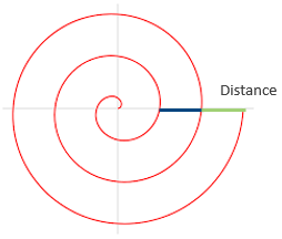
SPIRAL_LOOPdefines the number of loops (concentric spirals). Any single loop is a complete 360° spiral. Values less than 1.0 draw a partial spiral.
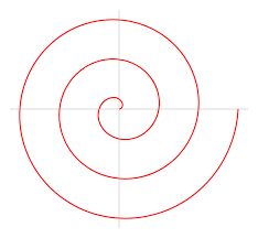
COEFFICENT_Bis the coefficient used to define the distance between the loops of the concentric spiral.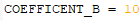
BOX_HEIGHTsets the height of the boxes (Y).BOX_WIDTHsets the width of the boxes (X).
Both are expressed in pixels.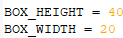

Set the distance of the loops and their numbers according to the size of the boxes. Wrong parameters setting can make the boxes overlap, especially inside the inner part of the spiral.
Running the Python script
Run the Spiral Oriented Sub Volume Python Script by pressing the Run Script button or pressing the F5 key.
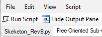
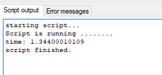
Note: Activate the Output Panel, if not already displayed. The status of the script execution (errors including) will be visualized here.
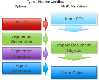
Building the analysis pipeline
The pipeline has to be created according to the user analysis requirements as well as the sample typology.
The sample labeling, the imaging technique (Fluorescence, EM, Tomography, bright-field ...) and the image characteristics are important to drive the pipeline setup.
The knowledge of the biological structures under evaluation, it’s behavior and the expected features' trend are also important as well. All the above information should be used to build a target driven pipeline.
To achieve the application note goals, only a couple of operators are mandatory, as described below:
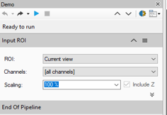
- Change the ROI operator parameters inside the Input ROI dialog.
-
![Input ROI panel: ROI 'Current time point', Channels '[all channels]', Scaling '100 %', Include Z checkbox](https://ariviskbdevwe.blob.core.windows.net/cdn/downloads/blobs/cb64625485e6d16c72b57a39b08c5e23.webp)
- A dropdown menu will open.
- Inside the dropdown menu, set the processing and analysis target space.
Following options are available:
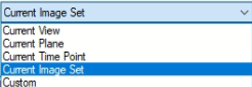
Current View: The selected Z plane and the viewer area will be processed.
Current Plane: The selected Z plane will be processed (XY).
Current Image Set: The complete dataset (XYZ and time) will be processed.
Current Time Point: The selected time point will be processed (XYZ).
Custom: Allows to mix the previous methods and expands the Input ROI dialog.
NOTE: Use the Custom option during setting and testing of the pipeline. Set a sub volume (XY, Planes, Time Points, channels) of your dataset on which to perform the trial. This will speed up the setting process.
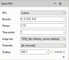
- Use the Custom option during setting and testing of the pipeline. Setting a sub volume of your dataset on which to perform the trial, will speed up the setting process. You have the following setting options:
Bounds: Sets the analysis area edges. The whole XY bounds, the viewing area or a custom space can be applied.
Planes: Sets the analysis planes range. A single plane, a range of planes or the whole stack can be selected.
Time Points: Sets the analysis time points range. A single TP, a range of TPs or the whole movie can be selected.
Channels: Sets the processing and analysis target channels. Selecting a single channel, all the operators in the pipeline will be forced to use it.
Scaling: Scales the dataset by reducing the size. The measurements will not be modified by the scaling factor.
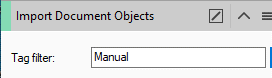
- Set the Import Document Objects operator, by selecting the Tag filter inside the Import Document Objects dialog .

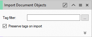
- The select tags dialog opens.
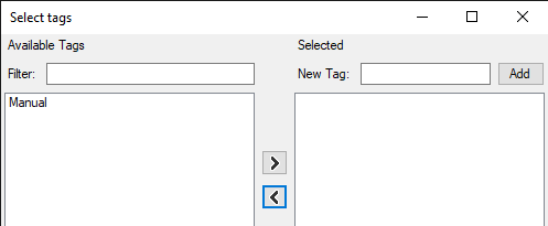
- Select the Manual TAG and use the right arrow button to move the TAG to the right table.
![Software Input ROI panel showing ROI set to 'Current view', Channels '[all channels]', Scaling 100%](https://ariviskbdevwe.blob.core.windows.net/cdn/downloads/blobs/7533d5b21c378bacc16dc8a838b47af4.webp)
- Add or remove optional operators inside the pipeline.
- The Analysis Pipeline panel consists of two main areas. The Pipeline area and the Analysis Operations area.
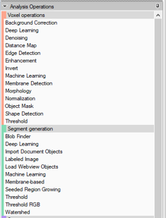
- Add the Operators to the pipeline in two possible ways:
1. Double-click on the Operator you wish to add to the current pipeline. The Operator will be inserted at the end of the group of operations to which it belongs. Voxel operations are positioned before the Segment generation meanwhile Store operations are put always at the end of the pipeline.
2. Drag and drop the Operator you wish to add to the current pipeline. The Operator will be automatically inserted in any place within the group of operations to which it belongs. NOTE: The Operator cannot be added during the pipeline execution. - To remove an Operator from the pipeline, press the X button located in the right side of the operator title bar.

Please refer to arivis Pro Help for more details.
Running the analysis Pipeline
The pipeline can be executed step by step (back and forth). This method allows to run and undo a single Operation. Either the arrow buttons or the Operation list can be used to go through the operators list.
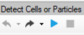
- Run the single operator.

- Optional: Undo the single operator.

Note: Undo the last operator executed if you need to change the operator settings. - Run the whole pipeline with no pauses.

- Optional: Stop the pipeline execution.

This icon, located on the right side of the operator title bar, shows the operator status.
Task running: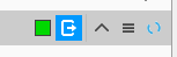
Task completed: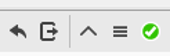
Viewing the results
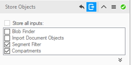
- Results (segments and measurements) will be stored in the dataset only if the Store Objects operator has been correctly set. Tick appropriately the option as shown below before complete the pipeline execution.
- Open the data table if not already visible.
- Measurements are now visible in the data table.
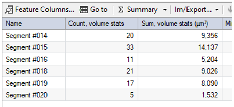
Note: The spots count in the single sub-region is shown in the data table. The empty sub-regions are not listed. To get the total spots count the group statistic feature must be used. 
Features can be added or removed from the data table using the Feature Column command.