ZEISS Microscopy Knowledge Base

Help

ZEISS Microscopy Knowledge Base

Creating Heat-Map – density distribution

This guide explains how to create a density distribution map, also called ”Heat-Map”. The script generates contiguous boxes in X,Y and Z directions that can be used as ROIs for further analysis (Compartmentalization, gradient distribution, etc.)

Opening the working dataset

Select Open... from the file menu.
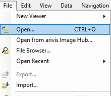
Select the dataset from the file browser.
The dataset is a multi dimensional, discrete, representation of your real sample volume. It can be structured as a Z series of planes (Optical sectioning) of multiple channels (dyes) in a temporal sequence of time points (located in several spatial positions).
Usually, the dataset shows a single experimental situation (a complete experiment can be composed by several datasets). The datasets are available as graphic files saved in plenty of file formats (standard formats as well as proprietary formats).
Note: The dataset is visualized according to the current rendering setting parameters. Refer to the arivis Pro Help for more details.

Software GUI with 3D volumetric rendering of green and red segmented objects on a grid, left-side tool panels and color scale

Loading the Python script

Open Python Script Editor. From the Extra menu, select Script Editor.
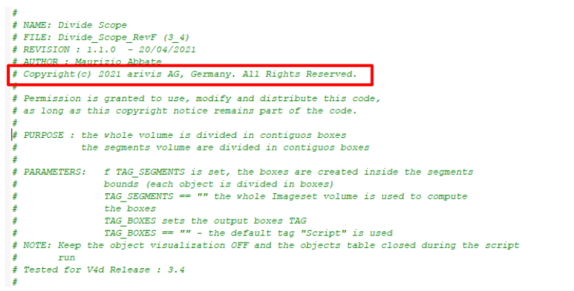
Load the Divide_Scope Python Script.
Note: The script name can change according to the new version released. The latest script is: DivideScope RevE (3_4).py.
Browse the folder on which the file has been saved.

Python script code usage rights:The user has the permission to use, modify and distribute this code, as long as this copyright notice remains part of the code itself: Copyright(c) 2021 arivis AG, Germany. All Rights Reserved.

Set the Script features

In order to define the contigues sub-regions (sampling volume) features, some parameters of the script should be adjusted to match your analysis needs. These parameters are located in the code area labeled as USER SETTING.

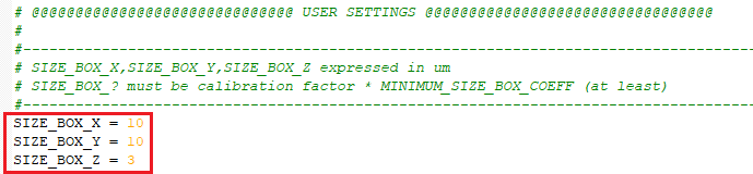
Code screenshot titled USER SETTINGS showing SIZE_BOX_X = 10, SIZE_BOX_Y = 10, SIZE_BOX_Z = 3

SIZE_BOX_X : Set the X sub-volume size.

SIZE_BOX_Y : Set the Y sub-volume size.

SIZE_BOX_Z : Set the Z sub-volume size.

All the values are expressed in metric units (µm).

If one of the box dimensions is bigger than the correspondent volume size, the script will not be executed and an error message is issued.

Only the parameters located in the USER SETTING area can be modified. Don’t change any other number, definition or text in the code outside this dedicated area.

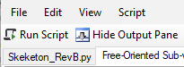
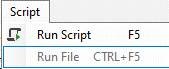
Running the Python script

Run the DivideScope RevE (3_4) Python Script by pressing the Run Script button or pressing the F5 key.

Toolbar with Run Script button and Hide Output Pane, tabs labeled Skeketon_RevB.py and Free-Oriented Sub-...

Script menu showing Run Script F5 and Run File CTRL+F5 options

Note: Activate the Output Panel, if not already displayed. The status of the script execution (errors including) will be visualized here.

This is the script result, a 3D matrix of sub-volumes:

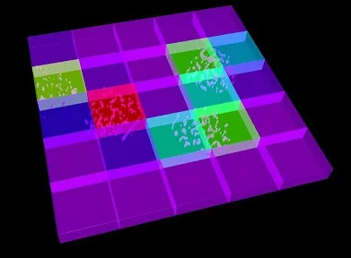
Tilted purple grid platform with raised translucent green, cyan and red tiles showing white flecks on black background

The sub-volumes segments are shown in the objects table using the TAG Script.

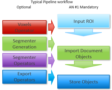
Building the analysis pipeline

The pipeline has to be created according to the user analysis requirements as well as the sample typology.

The sample labeling, the imaging technique (Fluorescence, EM, Tomography, bright-field ...) and the image characteristics are important to drive the pipeline setup.

The knowledge of the biological structures under evaluation, it’s behavior and the expected features' trend are also important as well. All the above information should be used to build a target driven pipeline.

To achieve the application note goals, only a couple of operators are mandatory, as described below:

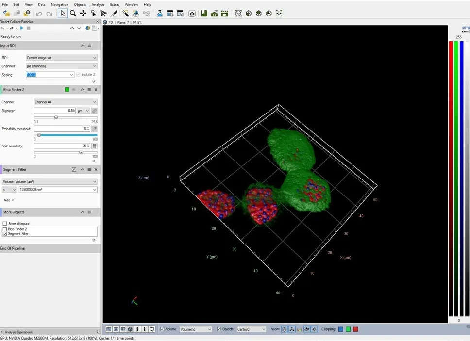
Pipeline diagram: optional left operators point to mandatory Input ROI, then Import Document Objects, then Store Objects

Change the ROI operator parameters inside the Input ROI dialog.
A dropdown menu will open.
Inside the dropdown menu, set the processing and analysis target space.

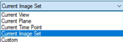
Following options are available:
Current View: The selected Z plane and the viewer area will be processed.
Current Plane: The selected Z plane will be processed (XY).
Current Image Set: The complete dataset (XYZ and time) will be processed.
Current Time Point: The selected time point will be processed (XYZ).
Custom: Allows to mix the previous methods and expands the Input ROI dialog.
NOTE: Use the Custom option during setting and testing of the pipeline. Set a sub volume (XY, Planes, Time Points, channels) of your dataset on which to perform the trial. This will speed up the setting process.
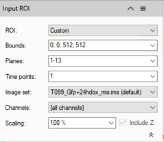
Use the Custom option during setting and testing of the pipeline. Setting a sub volume of your dataset on which to perform the trial, will speed up the setting process. You have the following setting options:
Bounds: Sets the analysis area edges. The whole XY bounds, the viewing area or a custom space can be applied.

Planes: Sets the analysis planes range. A single plane, a range of planes or the whole stack can be selected.

Time Points: Sets the analysis time points range. A single TP, a range of TPs or the whole movie can be selected.

Channels: Sets the processing and analysis target channels. Selecting a single channel, all the operators in the pipeline will be forced to use it.

Scaling: Scales the dataset by reducing the size. The measurements will not be modified by the scaling factor.
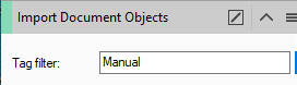
Set the Import Document Objects operator, by selecting the Tag filter inside the Import Document Objects dialog .
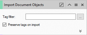
The select tags dialog opens.
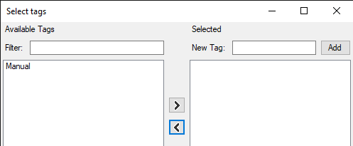
Select the Manual TAG and use the right arrow button to move the TAG to the right table.
Add or remove optional operators inside the pipeline.
The Analysis Pipeline panel consists of two main areas. The Pipeline area and the Analysis Operations area.
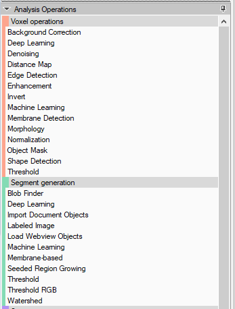
Add the Operators to the pipeline in two possible ways:
1. Double-click on the Operator you wish to add to the current pipeline. The Operator will be inserted at the end of the group of operations to which it belongs. Voxel operations are positioned before the Segment generation meanwhile Store operations are put always at the end of the pipeline.
2. Drag and drop the Operator you wish to add to the current pipeline. The Operator will be automatically inserted in any place within the group of operations to which it belongs. NOTE: The Operator cannot be added during the pipeline execution.
To remove an Operator from the pipeline, press the X button located in the right side of the operator title bar.

Please refer to arivis Pro Help for more details.

Running the analysis Pipeline

The pipeline can be executed step by step (back and forth). This method allows to run and undo a single Operation. Either the arrow buttons or the Operation list can be used to go through the operators list.

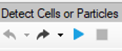
Toolbar titled 'Detect Cells or Particles' showing arrows, dropdown, blue play and gray stop square

Run the single operator.
Optional: Undo the single operator.

Note: Undo the last operator executed if you need to change the operator settings.
Run the whole pipeline with no pauses.
Optional: Stop the pipeline execution.

This icon, located on the right side of the operator title bar, shows the operator status.

Task running:
Grey bar with icons: green square, blue square with white arrow, up caret, menu, cyan circular arrows

Task completed:
Grey bar icons: left arrow, blue square with white arrow, up caret, menu, green circle with white check

Viewing the results

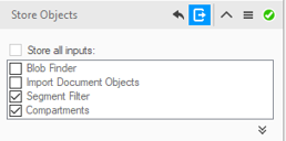
Results (segments and measurements) will be stored in the dataset only if the Store Objects operator has been correctly set. Tick appropriately the option as shown below before complete the pipeline execution.

Store Objects dialog with checkboxes for Blob Finder, Import Document Objects, Segment Filter (checked), Compartments (checked)

Open the data table if not already visible.
Measurements are now visible in the data table.

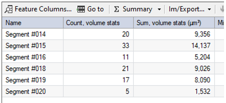
Note: The spots count in the single sub-region is shown in the data table. The empty sub-regions are not listed. To get the total spots count the group statistic feature must be used.

Features can be added or removed from the data table using the Feature Column command.
Toolbar area showing Feature Columns..., Go to, Σ Summary and Im/Export... controls