Performing objects density (heat-map) and object distribution gradient plotting (profile)
This guide explains how to perform the Objects density distribution analysis per volume unit (heat-map).
The same workflow can be used to evaluate the Objects count' distribution gradient along a specific direction (gradient profile). The application uses a Python script to create the contiguous sub-regions (sampling volume) and a pipeline to count the objects and to compute its density per volume unit (single sub-region) or the distribution along the longest direction of the sub-regions structure.
The evaluated Objects can be any biological structures like Cells, Nuclei, Neurons, as well as any small structures like Vesicles, Protein clusters, Mitochondria, and etcetera. The sampling volume can describe and limiting any anatomical regions inside the sample.
The unique limits is related to the sampling volume shape, only regular 3D boxes are available.

See also
Opening the working dataset
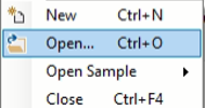
- Select the Open... item from the file menu.
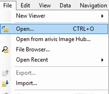
- Select the dataset from the file browser.
Note: The dataset is visualized according to the current rendering setting parameters. Refer to the arivis Pro Help for more details.
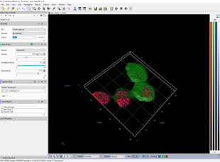
The dataset is a multi dimensional, discrete, representation of your real sample volume. It can be structured as a Z series of planes (Optical sectioning) of multiple channels (dyes) in a temporal sequence of time points (located in several spatial positions).
Usually, the dataset shows a single experimental situation (a complete experiment can be composed by several datasets). The datasets are available as graphic files saved in plenty of file formats (standard formats as well as proprietary formats).
Drawing the reference ROI
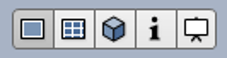
- Switch the Viewing area from 4D to 2D view mode.
- Select the Draw Objects tool.
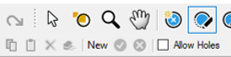
- Select the Brush tool.
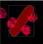
- Draw the 2D ROI over any Z plane. Use the Erase Brush to correct the ROI if necessary.
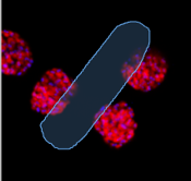
- Press the green icon to confirm the ROI.
The TAG Manual is now available in the data table.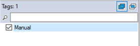
Loading the Python script
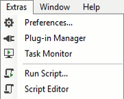
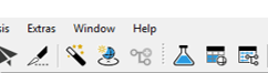
- Open Python Script Editor. From the Extra menu, select the Script Editor item.
- Load the Free-Oriented Sub-volume Python Script.
- Browse the folder on which the file has been saved.
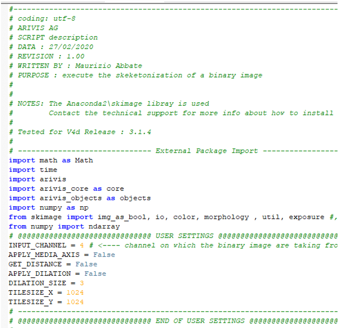
Only the parameters located in the USER SETTING area can be modified. Don’t change any other number, definition or text in the code outside this dedicated area.
Setting the script features
To define the contiguous sub-regions (sampling volume) features, few parameters of the script should be adjusted to match your analysis needs. These parameters are located in the code area labeled as USER SETTING.
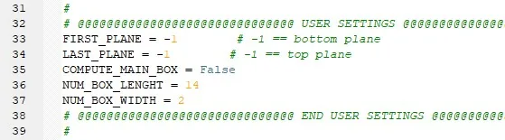
- Set the Z planes range.
FIRST_PLANE defines the lower Z plane of the sub-regions ROI.
LAST_PLANE defines the higher Z plane of the sub-regions ROI.
The values of -1 set the Z planes range equal to the whole volume depth (total number of Z Planes available).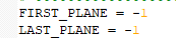
- COMPUTE_MAIN_BOX = True enables the creation of an additional ROI having the same sizes of the total subregions ROI size.
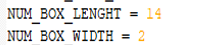
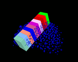
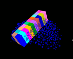
- NUM_BOX_LENGHT defines the number of sub-regions along the main axis (the longest one). NUM_BOX_WIDTH defines the number of sub-regions along the minor axis (the shortest one).
Note: Set the number of sub-regions accordingly to the total size of the reference ROI. Don’t create boxes too small.
Examples:
NUM_BOX_LENGHT = 10
NUM_BOX_WIDTH = 1
NUM_BOX_LENGHT = 10
NUM_BOX_WIDTH = 2
Running the Python script
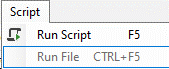
Run the Free-Oriented Sub-volume Python Script pressing the Run Script button or pressing the F5 key.
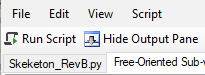
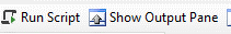
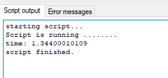
Note: Activate, if not already displayed, the Output Panel. The status of the script execution (errors including) will be visualized here.
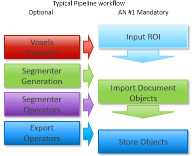
Building the analysis Pipeline
The pipeline have to be created according to the user analysis requirements as well as the sample typology. The sample labeling, the imaging technique (Fluorescence, EM, Tomography, bright-field ...) and the image characteristics are important to drive the pipeline setup. The knowledge of the biological structures under evaluation, it’s behavior and the expected features' trend are also important as well. All the above information should be used to build a target driven pipeline. The achieve the application note goals, only a couple of operators are mandatory. As described here below.
The Operators are grouped in several categories. Each category includes the functions that perform specific tasks, ordered by their usage. Here below a short summary.
|
Purpose |
Application |
|
|---|---|---|
|
Voxels Operator |
The group includes the operators that interact directly with the voxels. Typically, spatial filters, Intensity normalization, intensity range equalization and so on. |
Sample Noise removal, background subtraction, Intensity disomogenity correction, details enhancement, edges detection (e.g. membrane), morphological math. |
|
Segmenter Generation |
The group includes the threshold operators used to detect and create the segments. Automatic and manual method, machine learning approach, watershed and proprietary algorithms are available. |
Structures identification. Nuclei, Neurons, small spots (Blob Finder), Cells, Vessels, Filaments (Watershed, Region Growing) or microstructures (Machine learning) can be detected using the appropriate method or a combination of them. |
|
Segmenter Operators |
The group includes the operators that interact directly with the segments. Feature filtering, morphology, Compartmentalization, distance measurements and more can be applied. |
Objects colocalization, object classification by features, objects merging or splitting, objects grouping, objects parent/child relationship and even more. |
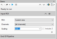
- Change the Input ROI operator parameters.
![Input ROI panel: ROI 'Current time point', Channels '[all channels]', Scaling '100 %', Include Z checkbox](https://ariviskbdevwe.blob.core.windows.net/cdn/downloads/blobs/cb64625485e6d16c72b57a39b08c5e23.webp)
- Sets the processing and analysis target space.
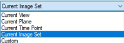
Current View: The selected Z plane and the viewer area are processed.
Current Plane: The selected Z plane is processed (XY).
Current Time Point: The selected time point is processed (XYZ).
Current Image Set: The complete dataset (XYZ and time) is processed.
Custom: Allows to mix the previous methods.
Note: Use the Custom option during the pipeline setting and testing. Set a sub volume (XY, Planes, Time Points, channels) of your dataset on which perform the trial. This will speed up the setting process. - Expand the Input ROI dialog.

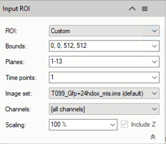
Bounds: Sets the analysis area edges. The whole XY bounds, the viewing area or a custom space can be applied.
Planes: Sets the analysis planes range. A single plane, a range of planes or the whole stack can be selected.
Time Points: Sets the analysis time points range. A single TP, a range of TPs or the whole movie can be selected. - Channels: Sets the processing and analysis target channels. Selecting a single channel, all the operators in the pipeline will be forced to use it.
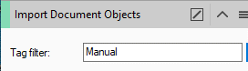
Scaling: It scale the dataset reducing the size. The measurements will not be modified by the scaling factor. - Set the Import Document Objects operator and select the TAG filter.
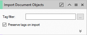
- Click on the Manual TAG.
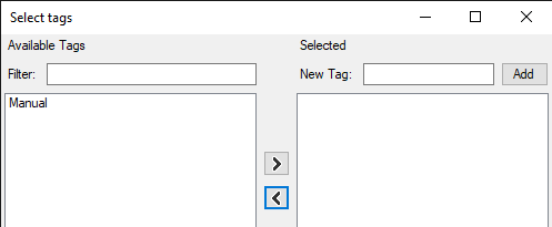
- Use the right arrow button to move the TAG on the right table.
![Software Input ROI panel showing ROI set to 'Current view', Channels '[all channels]', Scaling 100%](https://ariviskbdevwe.blob.core.windows.net/cdn/downloads/blobs/7533d5b21c378bacc16dc8a838b47af4.webp)
- Add or remove optional operators inside the pipeline.
The Analysis Pipeline panel consists of two main areas. The Pipeline area and the analysis operations list area.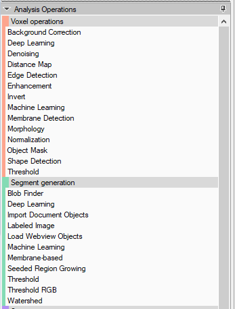
The Operators can be added to Pipeline in two ways: - Double click on the Operator you wish to add to the current Pipeline. The Operator will be inserted at the end of the group of operations to which it belongs. Voxel Operations are positioned before the Segment generation meanwhile Store operations are put always at the end of the Pipeline.
- Drag and drop the Operator you wish to add to the current Pipeline. The Operator will be automatically inserted in any place within the group of operations to which it belongs. The Operator cannot be added during the Pipeline execution.
- To remove an Operator from the Pipeline, press the X button located in the right side of the operator title bar.

Refer to the arivis Pro Help for more details.
Running the analysis Pipeline
The pipeline can be executed step by step (back and forth). This method allows to run and undo a single Operation. Either the arrow buttons or the Operation list can be used to go through the operators list.
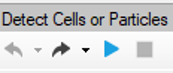
- Run the single operator.

- Optional: Undo the single operator.

Note: Undo the last operator executed if you need to change the operator settings. - Run the whole pipeline with no pauses.

- Optional: Stop the pipeline execution.

This icon, located on the right side of the operator title bar, shows the operator status.
Task running:
Task completed:
Viewing the results
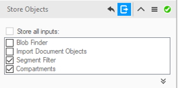
- Results (segments and measurements) will be stored in the dataset only if the Store Objects operator has been correctly set. Tick the option as shown below before complete the pipeline execution.
- Open the data table if not already visible.
- Measurements are now visible in the data table.
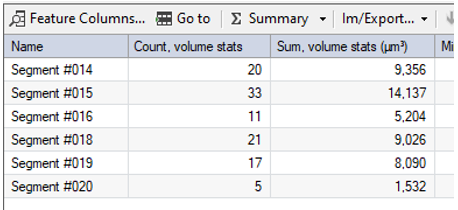
Note: The spots count in the single sub-region is shown in the data table. The empty sub-regions are not listed. To get the total spots count the group statistic feature must be used. 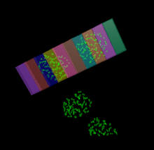
Features can be added or removed from the data table using the Feature Column command.