How does arivis handle large datasets
arivis solutions are known for their ability to handle large datasets. This article explains in a little more detail why and how this is done.
See also
How do computers process image data?
Most people are familiar with the basic concept that computers deal with binary data, where every morsel of information that is stored and processed in a computer is reduced to a series of 1s and 0s. However, few truly understand how that affects many aspects of how computers store and process data. A complete explanation of the intricacies of computer data processing is much too large for the scope of this article, but some basic explanation may help clarify why arivis solutions do the things they do the way they are done.
The first thing to consider is how images are stored. Most will be familiar with the concept of Pixels. A pixel is very simply an intensity value for a specific point in a dataset. 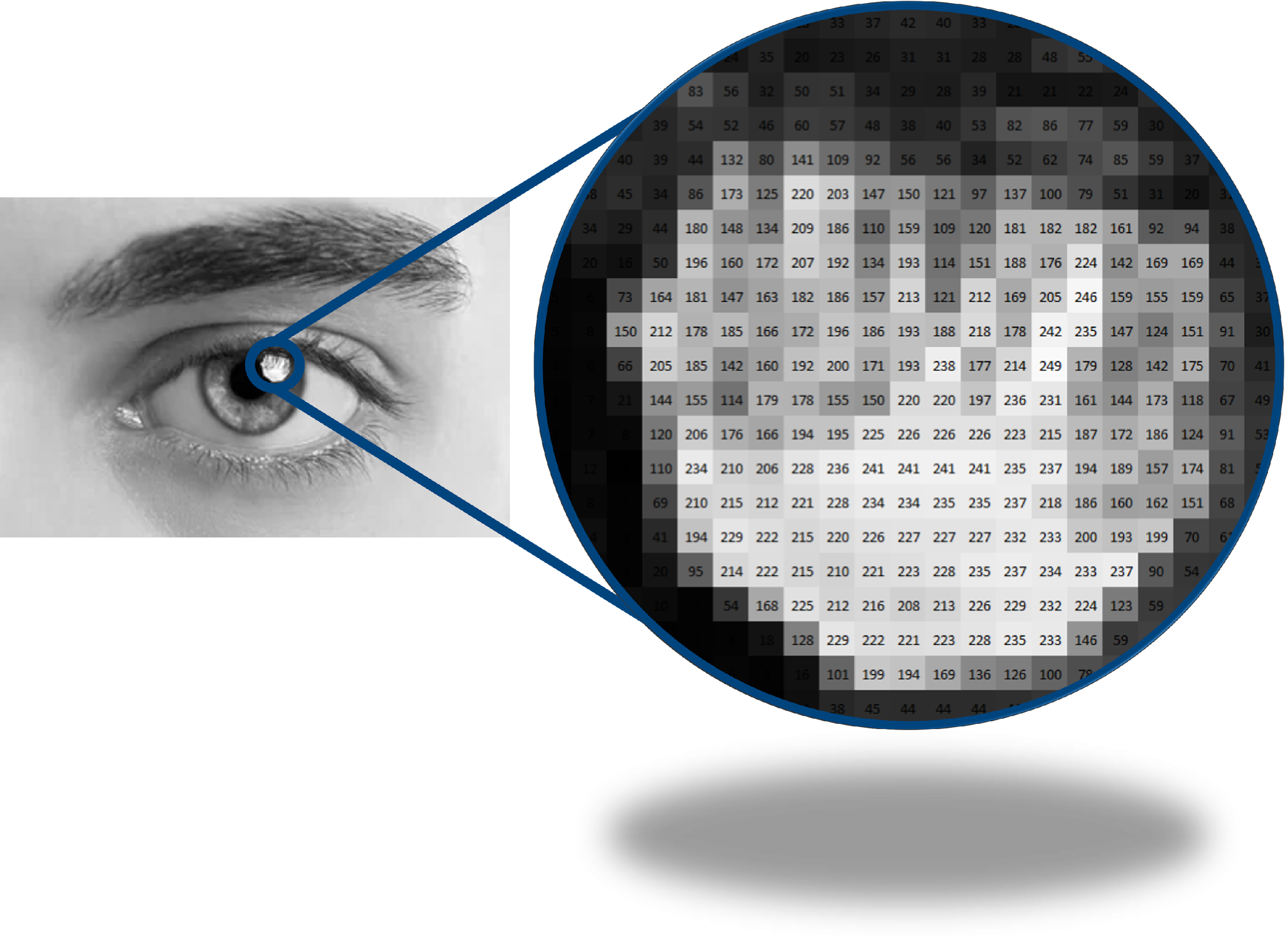
Looking at the example above, most human beings will, with little thought or effort, recognize a picture of an eye. But the data that is stored and displayed by the computer is a matrix of intensity values. What imaging software does is translate the numbers representing intensity values stored in the image file and display them as intensities on the screen for the purpose of visualization, or apply rules to individual pixels based on those intensity values to identify specific patterns like recognizing objects. To translate it into a more familiar concept, an image is essentially a spreadsheet of intensity values.
Now, to come back to the idea of computers as binary machines that process 1s and 0s, these pixels values need to be stored in a way that makes sense to the computer. The smallest amount of information that a computer can process is called a bit. It is a value that can be either on or off, 1 or 0. Of course, when talking about intensity values, 1 or 0 is a very narrow range of possibilities. So, instead of using just one bit of data to store a pixel, we will use multiple bits. So, for a 2-bit image, each pixel would be represented by two bits. Therefore the completer range of possibilities would be 00, 01, 10, and 11. This gives us 4 degrees of variation. Each time we add a bit to our data structure we double the range of possible values. The more bits we use, the more degrees of separation we have between the minimum and maximum value.
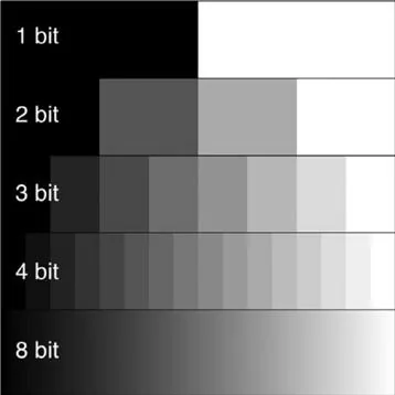
But each bit also represents a certain amount of computing resource used to store and process the data contained therein. So, for example, an 8bit image gives us 2^8 degrees of intensity variation for intensities between 0 and 255, and requires 8 bits or one byte per pixel in the image to store the file. In contrast, a 16-bit image gives us 2^16 degrees of variations (intensities between 0 and 65535), but also requires twice as much space on the disk and twice much processing resources as the 8-bit image since we are using twice as many bits to store and process the data.
This is important because all the image processing will be done by the computer, which has limited resources, and the data that is being processed needs to be held in the system's memory (RAM) for it to be available to the CPU. Moreover, the memory not only needs to hold the data the CPU is processing, but also the result of those operations, meaning that the computer really needs at least twice as much RAM as the data we are trying to process.
Typically in data processing, when an application opens a file, the entirety of that file's data is loaded into the system memory. Any processing on that image then outputs the results to the memory, and when the application closes only the necessary information is written back to the hard disk, either as a new file or modifications to the existing files. The problem with this approach comes when the files to be processed grow beyond the available memory. This is a very common problem in imaging as it is very easy when acquiring multidimensional datasets to generate files that are significantly larger than the available memory. Remember that each pixel usually represents 1 or 2 bytes of data. If we use a 1 million pixel imaging sensor, each image will represent 1/2 megabyte of data. If we acquire a Z-stack, we can multiply that by the number of planes in the stack. If we acquire multiple channels, as is common in fluorescence microscopy, we multiply the size of the dataset by the number of channels. If we want to measure changes over time we need to capture multiple time points. Each time we multiply the size of any of these dimensions we also multiply the size of the dataset by the same factor. It is relatively trivial in today's microscopy environment to generate datasets that represent several Terabytes of data.
So how does Vision4D work with my microscopy images?
Simply put, we don't. At least not directly. arivis Vision4D doesn't open any file in formats other than SIS. This means that to view and process your images we must first import them. To import a file into an SIS file we can simply drag and drop any supported file into an open viewer or our stand-alone SIS importer to start the import process. More details on the importing process can be found in the Getting Started user guide in the arivis Vision4D help menu.
Once imported, the original file can be kept as backup storage for the raw data and the SIS file can be used as a working document for visualization and analysis. The importing process will, in most cases, automatically read and copy all the relevant image metadata (calibration, channel colours, time intervals etc). If some of the metadata is missing for any reason it can easily be updated and stored in the SIS file. SIS files support a range of storage features, including:
- Calibration information
- Time information
- Visualization parameters (colors, display range, LUTs)
- 3D Bookmarks (including opacity settings, clipping plane settings, 4D zoom and location...)
- Measurements (including lines, segments, tracks etc)
- Version history, allowing for undos even after closing and saving a file
- Original file metadata not normally used in image analysis (e.g. microscope parameters like laser power, lens characteristics, camera details etc)
Because the original file is left unchanged, users can work with SIS files in arivis Vision4D and VisionVR with full confidence that the original data is safe, that changes to the SIS file are reversible, and that the imported file can be opened and processed on virtually any computer that has enough storage space to hold the data.