Using intensity range and visualization settings
This guide explains how to perform a correct intensity range setting and all the related adjustment operations needed to improve the image visualization.
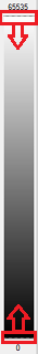
Color scalebar
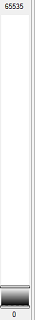
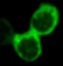
arivis Vision4D User Interface shows a Color Bar for each channel present in the dataset (The channel visibility must be set ON). The Color Bar usage has several purposes, one of them is the Dynamic Range optimal mapping with respect to the Display Range.
By dragging the top and bottom slider along the Color Bar, the Dynamic Range can be freely set.
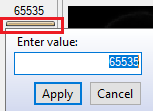
Right-Click on the slider. The top or bottom range value can be entered manually
The Dynamic range of each available channel can be adjusted independently.
The Dynamic range changing does not influence the intensity measurements.
By pressing the Auto button, arivis Vision4D computes the best Dynamic range setting based on the active Z plane intensity distribution (Histogram).

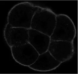
The active Z plane can be changed using the Navigator panel controls. Please refer to the (arivis Vision4D Help) for more details.
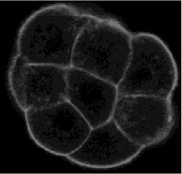
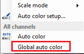
Right-Click on the Auto button. A pop-up menu is displayed. Select the Global auto color item to compute the best Dynamic Range setting based on all the Z planes Histograms.
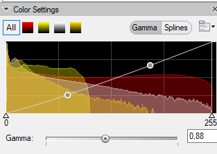
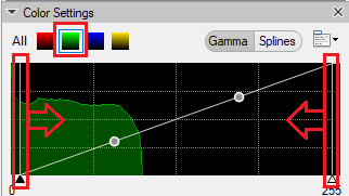
Color settings
Basically, the Color Settings panel allows to modify the Dynamic Range mapping as already shown above, but with a different approach. The range limits can be adjusted by dragging the lines at the beginning and end of the graph.
The target channel must be selected before moving the graph limits.
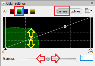
Gamma correction
Gamma is an important but seldom understood characteristic of virtually all digital imaging systems. It defines the non-linear relationship between a pixel's numerical value and its actual luminance. Without gamma, shades captured by digital devices wouldn't appear as they did to our eyes (on a standard monitor). Understanding how Gamma works can improve the image visualization and the details visibility. Our eyes do not perceive light the way the acquisition devices do. With an acquisition device, when twice the number of photons hit the sensor, it receives twice the signal (a "linear" relationship). That is not how our eyes work. Instead, we perceive twice the light as being only a fraction brighter — and increasingly so for higher light intensities (a "nonlinear" relationship).
Compared to an acquisition device, we are much more sensitive to changes in dark tones than we are to similar changes in bright tones. There is a biological reason for this peculiarity: it enables our vision to operate over a broader range of luminance. Otherwise, the typical range in brightness we encounter outdoors would be too overwhelming.
Below are some examples to clarify practically the Gamma concept:
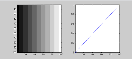
Gamma = 1.0
A "linear" transfer function.
This is the default value.
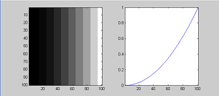
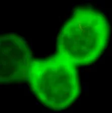
Gamma = 2.0
A “non-linear" transfer function.
The dark part of the range is expanded.
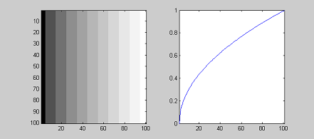
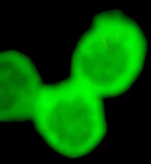
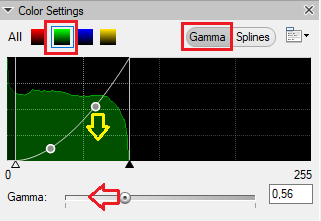
Gamma = 0,5
A “non-linear" transfer function.
The bright part of the range is expanded.
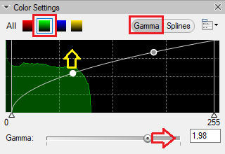
The Gamma value can be modified dragging the gamma slider left or right or directly inputting the value into the text box.
The curve shape can be also modified.
Gamma = 1.0 - "linear".
Gamma = 0,5 - “non-linear" The bright part of the range is expanded.
Gamma = 1,98 - “non-linear" The dark part of the range is expanded.
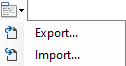
The Color Settings parameters can be exported / Imported as file.