Deconvolution
This module offers 3D deconvolution algorithms to enhance your 3D image stacks and methods for theoretical PSF. It uses efficient processing and significant performance gains via GPU acceleration with dedicated CUDA-compatible graphic cards, including support for multi-GPU. It also offers improvements in resolution down to 120 nm (depending on the imaging system) and is compatible with conventional widefield, Apotome, Lightsheet, confocal or multiphoton microscopes. Additionally to four primary methods, more than 15 published methods (e.g., Richardson-Lucy) can be employed by changing the parameters. Some functionality is generally available, for the full set of features you need the dedicated license for the module, see Licensing and Functionalities of Deconvolution.
Licensing and Functionalities of Deconvolution
Some basic functionality for deconvolution is generally available in the software, but the full Deconvolution functionality requires a license.
Basic functionality
The functionality generally available in ZEN includes:
- The 2D background removal function Deblurring which is based on the nearest neighbor algorithm.
- The Deconvolution (defaults) function, which offers three primary deconvolution methods that are automatically adapted to the type of instrument used to acquire the image.
Licensed Functionality
If you have licensed the functionality and activated it under Tools > Toolkit Manager, the following additional functionality is available:
- The additional and more advanced deconvolution method Constrained Iterative in the Deconvolution (defaults) function.
- GPU acceleration with dedicated CUDA-compatible graphic cards, including support for multi-GPU.
- The Deconvolution (adjustable) function, which offers access to all available function parameters and provides the necessary flexibility for demanding samples and sample conditions.
- The creation of a PSF with the PSF Wizard, a function offering a wizard to guide you through a series of steps to create a PSF from a z-stack image of multiple fluorescent beads. This function is recommended to create experimentally measured PSFs.
Basics of Deconvolution
Microscopy creates images of objects which should represent the nature of the object as well as possible. Fluorescent light, which emanates from the object, passes through the various optical elements of the beampath and eventually gets collected by the detector. Unfortunately, on the way to the detector the signal is changed in such a way, that the quality of the resulting image suffers. As a consequence, the image is never a 100% correct representation of the object. This effect is strongest seen in a classical widefield fluorescence microscopy which does in fact not offer any optical sectioning capability, but also exists to a different degree in optical sectioning microscope systems, e.g. Confocal, Lightsheet or ApoTome.
Fortunately, the dominant function which has this deleterious effect on the image, is based on the optical design principles of the light microscope and therefore well understood. We call this the point spread function (PSF) of the microscope system.
Deconvolution is a mathematical method which can reverse the effect of the PSF on the image and can therefore to a large extent restore the image to better represent the object. In the case of widefield imaging, Deconvolution can even convey optical sectioning properties to the result image allowing true three-dimensional restoration.
The following improvements can be obtained by using deconvolution:
- Denoising
- Removal of out of focus light -> deblurring, improved contrast
- Increasing signal to noise ratio by reassigning photons
- Restoration of sparsely sampled data
- Increase of resolution in X, Y and Z
As the object and the way, it was prepared, becomes part of the optical system during imaging, the largest variable to consider when doing deconvolution is the sample itself. Since the sample conditions can vary widely, information about the sample needs to be provided to the deconvolution function. The better the sample conditions are known, the better the outcome will be.
Deconvolution Methods in ZEN
|
Method |
Reference |
Settings |
Comments |
|---|---|---|---|
|
Nearest Neighbor |
K. Castleman, “Digital image processing”, Prentice Hall 1997 |
Algorithm (default): Nearest Neighbor |
Ad-hoc “2D de-blurring algorithm” focuses on subtraction of out of focus blur. |
|
Regularized Inverse also known as: Linear Least Squares |
For zero order g-difference: Schaefer et al. (2001) |
Algorithm (default): Regularized Inverse Filter Advanced settings > Regularization: Zero order |
Uses difference of observation and estimate as regularization term. |
|
Regularized Inverse also known as: Linear Least Squares |
For first order regularization, or Good’s roughness: Verveer et al. (1997) |
Algorithm: Regularized Inverse Advanced settings > Regularization: First order |
Uses Good’s roughness first derivative of estimate as regularization term. |
|
Regularized Inverse also known as: Linear Least Squares In conjunction with structured illumination microscopy (ApoTome) |
Schaefer et al. (2006) Schaefer et al. (tbs) |
Algorithm: Regularized Inverse Advanced settings > Regularization: Zero/First order |
Patented method for maximum exploitation of ApoTome raw images. |
|
Fast Iterative Also known as: Meinel Algorithm Gold Meinel |
Meinel (1986) |
Algorithm (default): Fast Iterative Advanced settings > Likelihood: Poisson (Meinel) |
Classic, non-regularized Meinel algorithm. |
|
Fast Iterative Meinel Algorithm + Regularization: |
Meinel (1986), For zero order g-difference: Schaefer et al. (2001) |
Algorithm: Fast Iterative Advanced settings: - Likelihood: Poisson (Meinel) - Regularization: Zero order |
Regularized Meinel algorithm using g-difference (difference of observation and estimate) term. |
|
Fast Iterative Meinel Algorithm + |
Meinel (1986), Biggs (1998) |
Algorithm: Fast Iterative Advanced settings: - Likelihood: Poisson (Meinel) - Regularization: None/Zero order - Optimization: Numerical Gradient |
Meinel algorithm using a numerical gradient estimator as proposed by D. Biggs. |
|
Fast Iterative Also known as: Richardson Lucy (RL) Algorithm |
Richardson (1972) Lucy (1974) |
Algorithm: Fast Iterative Advanced settings > Likelihood: Poisson (Richardson, Lucy) |
Classic, original non-regularized Richardson Lucy algorithm. May need many more iterations than any other algorithm. |
|
Fast Iterative Also known as: Richardson Lucy Algorithm + |
Richardson (1972) Lucy (1974) Biggs (1998) |
Algorithm: Fast Iterative Advanced settings: - Likelihood: Poisson (Richardson, Lucy) - Optimization: Numerical Gradient |
Classic, original non-regularized Richardson Lucy algorithm. Improved rate of convergence. About a factor of 10 faster than RL using a numerical gradient estimator as proposed by D. Biggs. |
|
Constrained Iterative |
Verveer et al. (1997) Schaefer et al. (2001) |
Algorithm (default): Constrained Iterative Advanced settings: - Likelihood: Poisson - Regularization: Zero order |
Generic conjugate gradient restoration using squared estimate to impose positivity. Uses difference of observation and estimate as regularization term. |
|
Constrained Iterative |
Verveer et al. (1997) Schaefer et al. (2001) |
Algorithm: Constrained Iterative Advanced settings: - Likelihood: Poisson - Regularization: First order |
Generic conjugate gradient restoration using squared estimate to impose positivity. Uses Good’s roughness derivative operator as regularization term. |
|
Constrained Iterative |
Tikhonov (1977) Verveer et al. (1997) Schaefer et al. (2001) |
Algorithm: Constrained Iterative Advanced settings: - Likelihood: Poisson - Regularization: Second order |
Generic conjugate gradient restoration using squared estimate to impose positivity. Uses Tikhonov Miller Phillips second derivative operator as regularization term. |
|
Constrained Iterative |
Verveer et al. (1997) Schaefer et al. (2001) |
Algorithm: Constrained Iterative Advanced settings: - Likelihood: Gauss - Regularization: Zero order |
Generic conjugate gradient restoration using squared estimate to impose positivity. Uses difference of observation and estimate as regularization term. |
|
Constrained Iterative |
Verveer et al. (1997) Schaefer et al. (2001) |
Algorithm: Constrained Iterative Advanced settings: - Likelihood: Gauss - Regularization: First order |
Generic conjugate gradient restoration using squared estimate to impose positivity. Uses Good’s roughness derivative operator as regularization term. |
|
Constrained Iterative Also known as: ICTM Iterative Constrained Tikhonov Miller |
van der Voort et al. (1995) Verveer et al. (1997) Schaefer et al. (2001) |
Algorithm: Constrained Iterative Advanced settings: - Likelihood: Gauss - Regularization: Second order |
Generic conjugate gradient restoration using squared estimate to impose positivity. Uses Tikhonov Miller Phillips second derivative operator as regularization term. |
|
Constrained Iterative |
Verveer et al. (1997) Schaefer et al. (2001) |
Algorithm: Constrained Iterative Advanced settings: - Likelihood: Poisson/Gauss - Regularization: 0/1/2nd order - Optimization: Line search/Analytical |
Generic conjugate gradient restoration using squared estimate to impose positivity. Default for optimization is the fast analytical (Newton Raphson) method. Line search may be more accurate but is also much slower. |
Bibliography
Schaefer, L.H., Schuster, D. & Herz, H. Generalized accelerated maximum likelihood based image restoration approach applied to three-dimensional fluorescence microscopy, Journal of Microscopy, 2004 (2001), Pt. 2, 99-107 (PubMed).
Verveer, P.J. & Jovin, T.M. (1997) Efficient superresolution restoration algorithms using maximum a posteriori estimations with application to fluorescence microscopy. J. Opt. Soc. Am. A, 14, 1696-1706.
Meinel E.S., Origins of linear and nonlinear recursive restoration algorithms, J. Opt. Soc. Am. A., 1986, 3 (6): 787-799.
Biggs, D.S.C. 1998. Accelerated Iterative Blind Deconvolution. Ph.D. Thesis, University of Auckland, New Zealand.
Schaefer, L.H. & Schuster, D. Structured illumination microscopy: improved spatial resolution using regularized inverse filtering, Proceedings of the FOM 2006, Perth, Australia.
Lucy L.B., An iterative technique for the rectification of observed distributions, Astron. J., 1974, 79: 745-754.
Richardson W.H., Bayesian-based iterative method of image restoration, J. Opt. Soc. Am., 1972, 62 (6): 55-59.
van der Voort, H. T. M. and Strasters, K. C. (1995) Restoration of confocal images for quantitative image analysis. J. Microsc., 178, 165–181.
Tikhonov, A.N. & Arsenin, V.Y. (1977) Solutions of Ill Posed Problems. Wiley, New York.
Performing Deconvolution Using Default Values
Successful deconvolution depends mainly on good image quality, knowledge about the optical parameters of the sample and detailed knowledge about the type of instrument used for image acquisition. While information about the used instrument type can be easily extracted from the image metadata, optical parameters of the sample might not be known and the image quality can vary widely. Many parameters are available for deconvolution which allow you to make corrections to the image quality and adjust the algorithms to match the various optical conditions such as coverslip type or the medium, in which the sample is embedded. This wide range of parameters can be overwhelming.
With the Deconvolution (defaults) method, good initial results are achieved by using a carefully preselected set of default parameters. The parameters are automatically adapted to the following instrument types: widefield, confocal, lightsheet and ApoTome.
While these parameters usually give nice results, there are cases where further parameter changes are necessary, e.g., activating and using spherical aberration correction. In such cases, you should use the Deconvolution (adjustable) method, see Performing Configurable Deconvolution.
- You are on the Processing tab.
- You have acquired or opened a fluorescence image on which you wish to perform deconvolution.
- All tools are in Show All mode.
- In the Method tool, in the Deconvolution group, select Deconvolution (defaults).
- Open the Parameters tool.
- Four different algorithms for deconvolution are displayed (Nearest Neighbor, Regularized Inverse Filter, Fast Iterative, Constrained Iterative), which you can apply to your image. Note that the Constrained Iterative algorithm is only available if you have the license for the Deconvolution module.
- Select an algorithm.
- Open the Input tool.
- If Set Input Automatically is activated, the currently active image is loaded as input image automatically. If the checkbox is deactivated, the container for the input image is empty. In this case continue with the next.
- Click on the empty image container.
- A list opens with preview images of all currently open images.
- Click on the image to which you want to apply deconvolution.
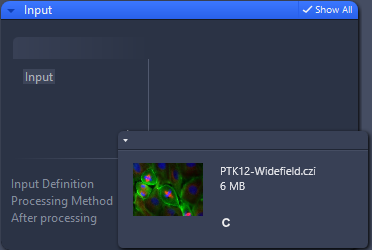
- The image is displayed in the image container and is as the input image for processing.
- Click Apply on the top of the Processing tab.
- Deconvolution is performed. A new image file is generated and opened automatically in the center screen area after processing. If you are satisfied with the result, save the processed image. Repeat deconvolution using the other default values to obtain different results. If you have expert knowledge, you can configure all the deconvolution settings yourself using the Deconvolution (adjustable) method.
Creating Deconvolution Settings
You can create settings for Deconvolution which can be saved, exported, and imported.
- Open the Processing tab and select the method Deconvolution (adjustable).
- In the Parameters window, activate Show All (if it is not already activated).
- In the Input window, select the desired image for the Deconvolution.
Note: If you use the settings for Direct Processing, use a test image acquired with the identical experiment settings you will be using when running the experiment with Direct Processing. - Click on the context menu button
 and select New from the drop-down list.
 - Enter a name for your settings and press Enter on your keyboard or click on the save button
 .
. - Configure your settings in the Deconvolution or PSF settings tab, see also Deconvolution tab and PSF Settings tab.
- Click on the context menu button and select Save.
- You have now created and saved a Deconvolution setting. You can load this setting into the Direct Processing tool to use it for a Direct Processing experiment.
GPU
The setting also saves the status of the GPU. If you create the setting on a machine without a GPU, export it, and import the setting on machine with GPU, the GPU will not be used. Therefore, the processing can be considerably slow. In this case, we recommend creating the setting directly on the machine where the processing is executed.
Exception for Direct Processing:
If you set up your experiment and your setting on an acquisition PC without a GPU, the processing PC will ignore the status and use the GPU (if available).
Creating a PSF - With Wizard and Without
The PSF Wizard combines two steps which are necessary for extracting experimental point spread functions (PSF) from Z-Stacks of subresolution fluorescent beads:
- A bead averaging step finds individual beads, presents them for inspection, allows you to select the ones you like and then creates an averaged combination of all selected beads. This stack shows a single bead which is, as a consequence of the averaging function, fairly free of noise.
- The averaged bead stack is then run through the Create PSF function which removes background and residual noise, correctly scales the PSF and also converts the stack into a 32-bit floating point format which is better suitable for the mathematical procedures used in deconvolution.
- You have acquired a z-stack image. For more information, see Measuring the PSF Using Subresolution Beads.
- You have the license for the Deconvolution module.
- The use of the PSF wizard is activated.
- On the Processing tab, select the function PSF Wizard.
- Use Wizard and Bad Pixel Correction are activated by default.
- On the top of the Processing tab, click Apply.
- The PSF wizard opens and guides you through the creation of the PSF.
- If the Use wizard checkbox deactivated, the function displays the parameters for Bead Averaging. Note that these parameters are only available in Show all mode. We recommend using the PSF wizard.
- The result of the wizard is a PSF file which you can use for deconvolution of images acquired under the same conditions.
This method determines the position of fluorescent beads in a z-stack image. If these beads are too close to one another, they are excluded from the calculation. Beads which are far enough apart from one another are combined into a single bead, from which it is then possible to calculate a PSF using the Create PSF function.
Description of the algorithm
This function consists of a series of steps before and after processing. The aim is to find beads that are far enough apart from one another. The processing steps are as follows:
- Select input image
- Image smoothing
- Segmentation
- Alignment of the center of the found beads
- Averaging of the beads
Measuring the PSF Using Subresolution Beads
Preparation
- The surface of coverslips is hydrophobic which means, liquid droplets do not spread out easily and beads tend to aggregate at the edges. For PSF measurements you want individually spread out beads.
- Bath the coverslips for 10 minutes in 100% ethanol.
- Use forceps to remove the coverslip. Shake off excess liquid and run through bunsen burner flame.
- This makes the surface slightly hydrophilic which means, the droplets and beads spread out easier.
- Ideally, use ZEISS coverslips with a defined thickness of 170 μm. However, coverslips and mounting media for bead measurements must be identical to the ones used for the sample, the image of which shall be deconvolved. Beads should have a diameter below the resolution limit of the objective, e.g. 0.175 µm. Smaller diameters are better, but smaller beads are dimmer and can therefore be difficult to locate on the cover slip.
- Tetraspeck beads from Thermo Fisher Scientific have the advantage of covering four colors which are frequently used in imaging research, but some batches can show rapid loss of fluorescence. Single color beads are typically brighter.
- Break up agglomerates by sonicating stock suspension in a waterbath for 20 minutes. Stocks suspensions are way too dense, so dilute 1:100 with 70% ethanol.
- Create further dilutions of 1:1.000 and 1:10.000 by adding 100 µl to 900µl 70% ethanol. Mix well using a Vortex mixer.
- Put one 5 µl drop for each dilution on a cover slip using a 20 µl Eppendorf pipette
- Let dry. This should take less than 5 minutes. You can speed it up by putting the cover slip on a warm surface.
- Put 10-20 µl mounting medium on the coverslip. For aqueous mounting media seal edges of coverslip with valap (1:1:1 mixture of vaseline, lanolin, paraffin), nailpolish or paraffin.
- In the next step, you acquire an image.
Imaging
- Locate the beads on the microscope (e.g. use a 20 x lens first, then move to 63x oil). Start at the 1:100 spot which should have tons of beads and be easy to find.
- When found, move to a sparser spot and try to find an area with a couple of single beads in the FOV. This can be tricky, but usually you will be able to find good areas if you keep looking around.
- Acquire a Z-stack of a suitable area, observing the following rules.
- No saturation. This can be tricky with LSM’s. Use 12-bit mode at least.
- Only fill the dynamic range in the histogram to about 80%.
- Make sure to focus up and down when setting up the exposure times to measure the exposure suitable for the bright bead center to avoid the risk of saturation.
- Set up the z-stack as follows: in the Z-stack tool, click on the Optimal button.
- This sets the distance according to Nyquist. For bead measurments further reduce the slice distance to about half of what Optimal suggests.
- Also, define the top and bottom of the stack in such a way that the airy disc of the beads cannot be distinguished any longer.
- When ready, save and name the image properly.
- Look at the result in OrthoView: Do you see spherical aberrations? Are the beads symmetrical? Are there enough individual beads in the stack? Is the background low enough?
Processing in ZEN Blue
- Use the PSF wizard (Processing/Deconvolution) to extract the PSF from the bead-z-stack. For more information, see Creating a PSF - With Wizard and Without.
- The PSF wizard guides you step by step through the necessary procedure.
- The result of the wizard is a PSF file which you use in deconvolution for images acquired under the same conditions.
Using Deconvolution in Direct Processing
- If you are using Direct Processing on different computers, you have connected acquisition and processing computer, see Connecting Acquisition Computer and Processing Computer.
- To ensure that the processing computer reads incoming files and starts the processing, on the Applications tab, in the Direct Processing tool, you have clicked Start Receiving. This is usually active by default.
- On the Acquisition tab, Direct Processing is activated. This activates the Auto Save tool as well.
- Depending on your settings, you have defined the folder where the acquired images are stored in the Direct Processing or the Auto Save tool. Use a folder to which the processing computer has access. For information about sharing a folder, see Sharing a Folder for Direct Processing.
- On the Acquisition tab, you have set up your experiment for image acquisition.
- If you want to use advanced settings created with the Deconvolution (adjustable) function, you have the settings available, see also Creating Deconvolution Settings.
- On the Acquisition tab, open the Direct Processing tool.
- If no Direct Processing settings were made before for the current experiment, a particular processing function is already preselected depending on your microscope, channel settings and licenses.
- From the Processing Function dropdown list, select Deconvolution.
- Select a deconvolution method. We recommend Excellent, slow (Constraint Iterative). If you want to use an advanced settings file you have created with the function Deconvolution (adjustable), activate Use Advanced Settings.
- A dropdown list is displayed under Load Setting created in the Deconvolution function.
- In the drop-down list, select your advanced settings for Deconvolution.
Note: Currently Direct Processing supports settings configured in the Deconvolution tab of the image processing function Deconvolution (adjustable) and some parameters of the PSF Settings tab. Especially parameters that rely on external data (like using external PSF) are not possible with Direct Processing. - Set up the experiment. For optimal processing efficiency, select the Full Z-Stack per channel option. This way, the processing can start as soon as a channel-z-stack has been completed. Keep in mind that for Colocalization studies better results might be achieved when the default All Channels per Slice is used, depending specific application and filter configuration.
- Click Start Experiment to run the experiment. Note: You can pause the processing. If you stop the experiment, requests that have been sent earlier by the acquisition computer are not processed. However, already processed images will be retained.
- The images are stored in the folder you have defined in the Auto Save or Direct Processing tool. When you abort the acquisition, the remote processing will not take place. In case you have set up several processing functions, only the acquired image and the final output image are stored.
- The processing computer reads incoming files and starts the processing. The path to the selected folder, the currently processed image as well as the images to be processed are displayed in the Direct Processing tool. The processed image is saved to the same folder specified in the Direct Processing tool. If the image name already exists in this folder, the new file is saved under a new name <oldName>-02.czi.
- To cancel the processing on the processing computer, on the Applications tab, in the Direct Processing tool, click Cancel Processing.
- Once processing is finished, you are notified on the acquisition PC and can open and view the acquired image as well as the processed image. This should be done on the processing computer, so that you can immediately start a new experiment on the acquisition computer. However, you can also automatically open the processed image on the acquisition PC with the respective setting in the Direct Processing tool on the Acquisition tab.
- When you open the image, in the Image View, on the Info view tab, information about the executed deconvolution is available. When Deconvolution is done through Direct Processing, the info about Deconvolution parameters shows the suffix online and the Convergence History graph. Additionally, general information about Direct Processing (e.g. the duration) is also available on the Info view tab of the processed image.
See also
Image Types Suitable for Deconvolution
Most types of microscope images could in principle be deconvolved. However, there are practical limitations, for example the image file sizes might be too large or imaging conditions might be dominated by effects other than blurring by the point spread function. If, for example, a sample has strong light scattering properties or if light is strongly absorbed by the sample, deconvolution becomes difficult or impossible.
Deconvolution works both in 2D as in 3D. The PSF is very small in 2D, so the improvements of deconvolving 2D images are usually not very significant. Its full power deconvolution can show when processing 3D image stacks which have been acquired according to the following general rules:
- Acquisition of images with enough pixel resolution by choosing objectives with numerical apertures >0.5 and using camera resolutions with small enough pixel sizes as recommended by the Nyquist criterion.
- Acquisition of Z-stacks with distance between individual planes not larger than recommended by the Nyquist criterion (2-fold oversampling of the theoretically resolvable information, Optimal button in the Z-stack tool).
- Acquisition of enough planes above and below the structure of interest. As a rule, acquiring about half the axial PSF size above and below is enough to also get restoration of the structures at the top and bottom of the structure of interest.
- Avoiding saturation of the detector.
- Choosing imaging conditions to avoid sample bleaching.
- Avoiding spherical aberrations by choosing objectives, which use an immersion medium with a refractive index as close as possible to the mounting medium of the sample (for example using water immersion objectives for cell cultures in aqueous medium).
- Choosing sample media with low background fluorescence (for example phenol red free culture media).
ZEN deconvolution is suitable for images from many different microscope types. The following list of image types have been tested and are supported by ZEN deconvolution:
|
Imaging modality |
Suitability for Deconvolution |
Comment |
|---|---|---|
|
Widefield fluorescence |
+++ |
Ideally choose objectives with a numerical aperture > 0.5. |
|
LSM confocal imaging detecting |
+++ |
Prerequisite is to have chosen a dye with the correct excitation and emission wavelengths before acquisition. |
|
LSM Lambda and Online Fingerprinting imaging modes detecting fluorescence |
++ |
Exact excitation and emission wavelengths are missing, need to be added on the PSF page before attempting deconvolution. |
|
2-Photon (NLO) imaging using NDD (Non-descanned detectors) |
+++ |
Excitation wavelength > emission wavelength. |
|
ApoTome fluorescence |
+++ |
Only ApoTome raw images should be deconvolved. |
|
Spinning disk confocal |
+ |
No spinning disk specific PSF model available, still can get good results when processing with a PSF according to standard confocal conditions (~1.2 airy units), or choose measured PSF. |
|
Lightsheet |
- |
Only single view deconvolution supported, image sizes might be challenging, best results for high NA objectives. |
|
Airyscan |
- |
Airyscan raw data deconvolution is currently not supported, deconvolving already processed images is not recommended. Use the Airyscan Joint Deconvolution method for deconvolving Airyscan raw data. |
|
Elyra |
- |
Currently not supported. |
|
Bright field transmitted light images |
- |
Not supported. |
|
Axio Scan.Z1 |
+ |
Can be used for fluorescence stacks, however, frequently file sizes are prohibitive. Also, ideally JPEG-XR compression should not be used. |
|
Celldiscoverer 7 |
+++ |
Very well suited due to objectives specialized for life cell imaging; recommended use of Direct Processing module to improve the workflow. |
Table of Default Parameter for Deconvolution
The following table lists the parameters which are used by default for widefield, confocal, lightsheet and ApoTome images.
|
Microscope Type |
Widefield |
Confocal |
Lightsheet |
ApoTome |
|---|---|---|---|---|
|
General Deconvolution Parameter Defaults |
||||
|
Normalization |
Auto |
Auto |
Auto |
Auto |
|
Background Correction |
Off |
Off |
Off |
Off |
|
Flicker Correction |
Off |
Off |
Off |
Off |
|
Decay Correction |
Off |
Off |
Off |
Off |
|
Hot Pixel Correction |
Off |
Off |
Off |
Off |
|
Constrained Iterative Specific Defaults |
||||
|
Strength (automatic, manual; range 0..10) |
Auto |
Auto |
Manual (str 5) |
Auto |
|
Likelihood |
Poisson |
Poisson |
Poisson |
— |
|
Regularization |
Zero Order |
First Order |
Zero Order |
— |
|
Optimization |
Analytical |
Line Search |
Analytical |
— |
|
First Estimate |
Input |
Mean |
Input |
— |
|
Maximum Number Of Iterations |
40 |
7 |
40 |
— |
|
Auto Stop Percentage |
0.1 |
0.1 |
0.1 |
— |
|
Fast Iterative Specific Defaults |
||||
|
Method |
Poisson/Meinel |
Poisson/Richardson Lucy |
Poisson/Meinel |
— |
|
Regularization |
None |
None |
None |
— |
|
Optimization |
None |
None |
None |
— |
|
First Estimate |
Input |
Mean |
Input |
— |
|
Maximum Number Of Iterations |
15 |
50 |
15 |
— |
|
AutoStop Percentage |
0.1 |
0.1 |
0.1 |
— |
|
Regularized Inverse Specific Defaults |
||||
|
Regularization |
Zero Order |
Zero Order |
Zero Order |
First Order |
ON THIS PAGE
- Deconvolution
- Licensing and Functionalities of Deconvolution
- Basics of Deconvolution
- Deconvolution Methods in ZEN
- Performing Deconvolution Using Default Values
- Creating Deconvolution Settings
- Creating a PSF - With Wizard and Without
- Measuring the PSF Using Subresolution Beads
- Using Deconvolution in Direct Processing
- Image Types Suitable for Deconvolution
- Table of Default Parameter for Deconvolution