ZEISS Microscopy Knowledge Base

Help

ZEISS Microscopy Knowledge Base

Direct Processing

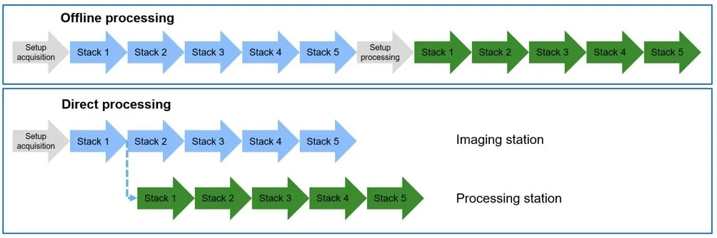
The development of microscopic techniques makes the data structure ever more complicated. In many cases, the raw data is large, time consuming to process and not needed at the end of the experiment. This module is designed to simplify the workflow to improve usability and to parallelize the acquisition and processing steps to save time.

During image acquisition using an acquisition PC, Direct Processing enables the user to select processing functions which are executed on a processing PC. Several different functions are available and you can define a sequence of functions (in a so-called pipeline), which are then executed sequentially one after another. Direct Processing starts to process the smallest processable entity as soon as its acquisition has been completed. In the case of deconvolution, this is typically a z-stack for one channel.

Diagram comparing 'Offline processing' and 'Direct processing' with blue imaging Stack arrows and green processing Stack arrows

Direct Processing allows an acquisition computer to communicate with a second PC (processing computer) connected via a network connection. The acquisition computer instructs the processing computer to process images as they are being acquired. Before you can use the module, you typically need to connect the two computers. As there are numerous ways, how computers can be set up to become networked, we can only give some general advice here. Contact your local IT administration for help on how to configure the computers in accordance to the local infrastructure.

One way is to connect the computer controlling the microscope system to a second computer via a direct ethernet connection. If Network Discovery is switched on, Windows 10 will directly support such a point to point connection. Create a shared folder which can be accessed from both computers. Since no other network traffic will use this connection, the whole bandwidth will be available for saving data directly from the acquisition computer to a shared folder on the processing computer. This is the most efficient way as the acquired data do not have to be copied off the acquisition computer after the acquisition has finished.
Alternatively, it is also possible, to use a processing computer which is already integrated into an existing network. Depending on the network type and the kind of experiments being done, the bandwidth might not be sufficient to directly stream data to the processing computer. In such cases, to not limit the throughput of the acquisition, it is advisable to let the acquisition computer acquire data to a local drive and instruct the processing computer where to look for the acquired data.

If no processing PC is available, it is also possible to configure the same acquisition PC for parallel processing steps, i.e. acquire and process images on the same workstation.

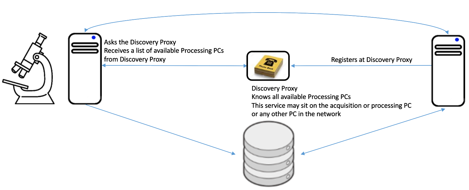
For a communication via network, it is possible to link both computers with a discovery proxy. The discovery proxy is a service where you can register all available processing computers and your acquisition computer can then ask this service for the list of these available PCs. You can also link the PCs without such a discovery service, for which you then need the IP address and/or network name of the processing computer. Note that such a use of a discovery proxy is primarily designed for configurations in which you have more than one processing PCs.

Network schematic showing microscope, acquisition and processing servers, a Discovery Proxy icon and database with labelled arrows — Schematic of the function of a discovery proxy

Overview Direct Processing

This overview shows you how to perform Direct Processing.

Before using the Direct Processing functionality on two computers, the acquisition and the processing computers need to be connected, see Connecting Acquisition Computer and Processing Computer.
On the acquisition computer, settings need to be defined, see Direct Processing Tool on Acquisition Tab.
On the acquisition computer, settings in the Auto Save tool need to be defined, see Defining Settings in the Auto Save Tool.
On the processing computer, the receiving needs to be activated, see Direct Processing Tool on Applications Tab.
Set up and run an experiment with Direct Processing, see Using Direct Processing.

Setting Up Your PC as Discovery Proxy

If you want to set up and use your computer as discovery proxy, take the following steps:

Open Tools > Options > Direct Processing.
Open the Setup Discovery Proxy Server section.
The options for setting up the discovery proxy open.
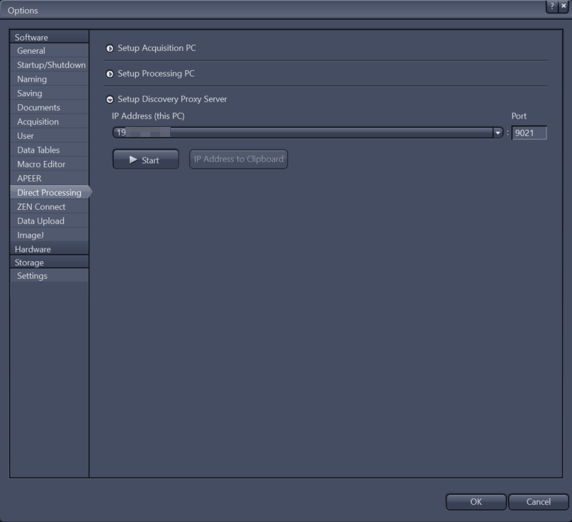
If your PC has several active network connections, under IP Address (this PC), select the IP address you want to use for the discovery proxy setup in the dropdown.
Click Start.
Click OK to close the Tools > Options dialog.

This computer is now set up and used as discovery proxy with the displayed IP address.

Defining Settings in the Auto Save Tool

Auto Save and ZEN Connect

If you have opened a ZEN Connect Project, the folder in the Auto Save tool is automatically set to the folder where the ZEN Connect project is saved. In this case you cannot change the folder for Auto Save. Also note that with an active ZEN Connect project you cannot select the upload to ZEN Data Storage.

Using Direct Processing and ZEN Data Storage

If you are using the ZEN Data Storage server as the location for storing your data, all acquisition and processing computers involved must have access to the transfer share defined in ZEN Data Storage.

Also note that the images are only uploaded to ZEN Data Storage after they are now longer open in ZEN.

When using the Direct Processing functionality, perform the following steps on the acquisition computer to define the settings in the Auto Save tool.

You have the Auto Save tool open on the Acquisition tab.

In the dropdown, select if you want to save the image(s) locally or upload them to ZEN Data Storage.
In the Folder field, specify the local directory, where acquired images should be stored. Make sure that it is a shared folder which can be accessed from both computers.
If you select Store in ZEN Data Storage Server, make sure that the processing computer is also connected to the same server. Optionally, you can define if the image should directly be shared with a particular collection.
If you want images to automatically be stored in a new subfolder named with the current date, activate Automatic Sub-Folder.
In the Name field, specify the file base name for the acquired images.
Activate Close CZI Image After Acquisition if you want to release the image from the acquisition computers memory.

Using Direct Processing

If you are using Direct Processing on different computers, you have connected acquisition and processing computer, see Connecting Acquisition Computer and Processing Computer.
To ensure that the processing computer reads incoming files and starts the processing, on the Applications tab, in the Direct Processing tool, you have clicked Start Receiving. This is usually active by default.
On the Acquisition tab, you have set up your experiment for image acquisition.
On the Acquisition tab, Direct Processing is activated. This activates the Auto Save tool as well.
Depending on your settings, you have defined the folder where the acquired images are stored in the Direct Processing or the Auto Save tool. Use a folder to which the processing computer has access. For information about sharing a folder, see Sharing a Folder for Direct Processing.

On the Acquisition tab, open the Direct Processing tool.
If no Direct Processing settings were made before for the current experiment, a particular processing function is already preselected depending on your microscope, channel settings and licenses.
From the Processing Function dropdown list, select the processing function you want to use.
The parameters of the function are displayed and the name of the function is displayed in the pipeline container.
Set all the parameters of the function for your experiment. For detailed information about the parameters refer to the descriptions of the individual image processing function.
To adjust the parameters individually for each channel of a multi-channel image, activate Adjust per Channel.
The tool displays all channels as a list and the currently selected channel is highlighted. For each channel you can use a dropdown to select whether to process it or to skip it (the channel is not processed and not part of the output image).
To add another function or several other ones, click Add Function.
A new container is added in the pipeline.
Select the next pipeline container, select a processing function from the dropdown, and set the parameters for each function.
You have added and set up a sequence of processing functions.
Click Start Experiment to run the experiment. Note: You can pause the processing. If you stop the experiment, requests that have been sent earlier by the acquisition computer are not processed. However, already processed images will be retained.
The images are stored in the folder you have defined in the Auto Save or Direct Processing tool. When you abort the acquisition, the remote processing will not take place. In case you have set up several processing functions, only the acquired image and the final output image are stored.
The processing computer reads incoming files and starts the processing. The path to the selected folder, the currently processed image as well as the images to be processed are displayed in the Direct Processing tool. The processed image is saved to the same folder specified in the Direct Processing tool. If the image name already exists in this folder, the new file is saved under a new name <oldName>-02.czi.
To cancel the processing on the processing computer, on the Applications tab, in the Direct Processing tool, click Cancel Processing.

Once processing is finished, you are notified on the acquisition PC and can open and view the acquired image as well as the processed image. This should be done on the processing computer, so that you can immediately start a new experiment on the acquisition computer. However, you can also automatically open the processed image on the acquisition PC with the respective setting in the Direct Processing tool on the Acquisition tab.
Information about Direct Processing (e.g. the duration) is available on the Info view tab of the processed image.

Using Direct Processing with Airyscan Processing

This function is only available if an Airyscan detector is available.
If you are using Direct Processing on different computers, you have connected acquisition and processing computer, see Connecting Acquisition Computer and Processing Computer.
To ensure that the processing computer reads incoming files and starts the processing, on the Applications tab, in the Direct Processing tool, you have clicked Start Receiving. This is usually active by default.
On the Acquisition tab, you have set up your experiment for image acquisition.
On the Acquisition tab, Direct Processing is activated. This activates the Auto Save tool as well.
Depending on your settings, you have defined the folder where the acquired images are stored in the Direct Processing or the Auto Save tool. Use a folder to which the processing computer has access. For information about sharing a folder, see Sharing a Folder for Direct Processing.

On the Acquisition tab, open the Direct Processing tool.
If no Direct Processing settings were made before for the current experiment, a particular processing function is already preselected depending on your microscope, channel settings and licenses.
In the Processing Function drop-down list, select Airyscan Processing.

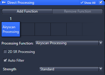
Note: If you uncheck the Auto Filter checkbox and activate Adjust per Channel, you can set the Super Resolution parameter in a channel specific manner.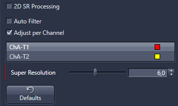
Select the desired settings for Airyscan Processing. For details how to use this function, see Airyscan Processing. Ideally, you have already checked the best parameters beforehand, using a sample image acquired under the same conditions as set up for the experiment.
Click Start Experiment to run the experiment.
Note: You can pause the processing. If you stop the experiment, requests that have been sent earlier by the acquisition computer are not processed. However, already processed images will be retained.
The images are stored in the folder you have defined in the Auto Save or Direct Processing tool. When you abort the acquisition, the remote Airyscan processing will not take place.
The processing computer reads incoming files and starts the Airyscan processing. The path to the selected folder, the currently processed image as well as the images to be processed are displayed in the Direct Processing tool. The processed image is saved to the same folder specified in the Direct Processing tool. If the image name already exists in this folder, the new file is saved under a new name <oldName>-02.czi.
To cancel the processing, click Cancel Processing.

Once processing is finished, you are notified on the acquisition PC and can open and view the acquired image as well as the processed images. This should be done on the processing computer so that you immediately can start a new experiment on the acquisition computer. However, you can also automatically open the processed image on the acquisition PC with the respective setting on the Direct Processing Tool on Acquisition Tab.
When you open the image in the Image View, information about the executed Airyscan processing is available on the Info view tab. Additionally, general information about Direct Processing (e.g. the duration) is also available on the Info view tab of the processed image.