Dynamics Profiler Calculations
Calculation of Concentration and Diffusion Coefficient
The diffusion coefficient D is calculated as indicated by the following formula:

The fluorofore concentration is given as:

- where
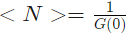
is an average number of molecules and NA is the Avogadro constant - and
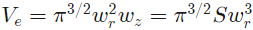
where S is the structural parameter.
Data Quality Criteria (CPM)
The data quality is estimated using CPM values:
|
Data Quality |
CPM Value |
|---|---|
|
Bad (red) |
Smaller than 1. |
|
Not bad (yellow) |
Between 1 and 3. |
|
Good (green) |
Higher than 3. |
Filters
Detrending Filter
The detrending filter is applied to remove the trend (e.g. due to the photo bleaching) from the experiment data. The detrended signal Id(t) is calculated as follows:
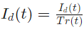
where the trend, Tr(t) is the gaussian smoothed signal:
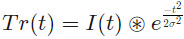
with 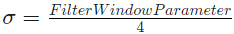
The FilterWindowParameter [ms] is set by the user.
Dust Filter
The dust filter allows you to remove high intensity peaks (e.g. caused by aggregated objects) from the experiment data. Calculations are done on the 500x down sampled signal data. For comparison, intensity data shown in the count rate chart is down sampled with factor 2000x. The data bin is classified as dust (filtered out) if the following criteria is fulfilled:
UserParameter * I(t) > Mean(I(t))
If both the detrending and dust filter are activated, the dust filter is applied after the detrending filter.
Fit Calculation
The unweighted fit of the correlation curve is done using the Levenberg-Marquart algorithm. Reduced chi2 is calculated as follows:

where Gt is the correlation curve value, Ft the fit value, N the number of correlation/fit values and DF the number of fit parameters.
Auto Correlation Fit Models
You can select one of the following models:
One Component 2D
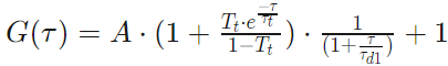
One Component 3D
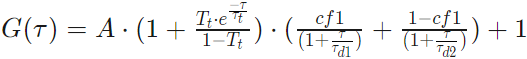
Two Component 2D
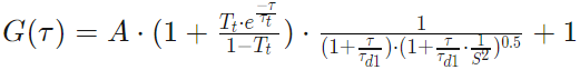
Two Component 3D

One Component Anomalous 2D
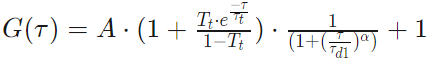
One Component Anomalous 3D
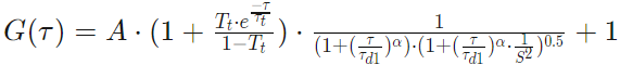
Parameters
The parameters used in the calculations are the following:
|
Parameter |
Description |
|---|---|
|
A |
The correlation amplitude. |
|
Tt |
The triplet fraction. |
|
Td1 |
The translational diffusion time. |
|
S |
The structural parameter. |
|
τt |
τt = 3µs is the fixed triplet relaxation time. |
|
cf1 |
The first component fraction. |
Normalization of Correlation Curves
Amplitude normalization of the correlation curves allows you to compare different correlation curves and see the differences in diffusion times between them.
If the fit of the correlation curves is already done, activating the amplitude normalization is done using the amplitude fit parameter. Selected correlation curves are rescaled that each selected curve has a correlation amplitude equal to 1 (corresponding number of molecules = 1).
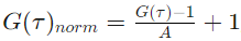
where A is a fitted amplitude.
In case no fit is done, correlation curves are normalized as follows:
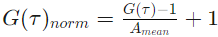
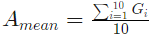
where Amean is the mean amplitude calculated over the first 10 points of the correlation curve:
Pair Correlation of Airyscan Fibers
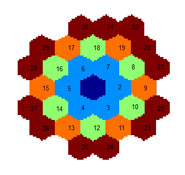
The pair correlation function (pCF) is a set of cross-correlations between the central fiber and all fibers located at a given distance from the center. For a better signal to noise ratio, cross-correlations are calculated in both directions and then averaged. The pCFs are used and displayed in the polar heatmaps of the Diffusion view.
The Diffusion view can display the data of two different sets of fibers. The group called Outer Elements comprises fibers with a slightly bigger distance from the center (blue element) and is illustrated with orange in the graphic below. The second group is called Inner Elements and comprises fibers with a slightly smaller distance from the center. They are illustrated with the green color in the graphic below.
|
Fiber Group |
Fibers |
|---|---|
|
Outer Elements |
Comprises fibers 9, 11, 13, 15, 17 and 19. |
|
Inner Elements |
Comprises fibers 8, 10, 12, 14, 16 and 18. |
ωr Calculation
The ωr is calculated with the following formula:
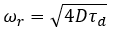
During the ωr calibration, τd is calculated in the one-component 3D diffusion model
and D (diffusion coefficient) needs to be provided and added in the ωr Calibration tab. The diffusion coefficients of commonly used dyes are already specified in a dropdown list. The following requirements need to be fulfilled in order to generate a suitable calibration file:
- Spot measurement duration of at least 60 seconds
- Time Resolution of 0.5 µs (ωr acquisition mode)
- The used dye concentration needs to be adjusted to match the expected FCS amplitude range (0.05 – 2)
- The emission wavelength of the selected dye should match the selected laser line
Four values are calculated and can be accessed by opening the calibration file with a text editor:
- W0Ring3: Effective radius of the observation spot (detector elements 1 to 19 binned together)
- W0Ring123: Average radius of the observation spot for a single detector element (average value for detector elements 1 to 19)
- R0Ring123: Effective distance between the detector elements for flow measurements
- StructuralParameter: Ratio between the observation spot waist in the axial and lateral direction
The generated ωr calibration file can be used in the Correlation Tools tab to replace the default ωr calibration values.
See also
Calculation of Autocorrelation Curve
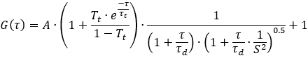
The Dynamics Profiler autocorrelation curve is calculated according to the formula:
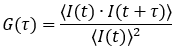
Correlation values are calculated for the lag times τ, commonly used in 16/8 multi-tau hardware correlators. This means the lag time τ is increased linearly with the τ =PixelDwellTime for the first 16 values. Then the lag time interval for τ is doubled, and the next eight lag times are calculated. The lag time interval is doubled after each next eight time lag values.
The very first correlation value, corresponding to the one PixelDwellTime, is skipped since it is biased due to correlation of the neighboring data points after low pass filter due to digitalization.