Software Autofocus

This module offers a configurable image based autofocus functionality that will search through a series of axially stepped images analyzing the “sharpness” of each. The z-value of the image returning the maximum sharpness is set as the new plane of observation.

The module requires the microscope to be fitted with a motorized Z-drive. It does not require a z-piezo actuator nor is the z-piezo used by the software autofocus (SWAF) in the current implementation. On the Acquisition or Locate tab the settings for the SWAF can be adjusted in the Software Autofocus tool. These can also be called (and tested) by clicking the Find Focus (AF) button on the main button bar on Acquisition tab. SWAF settings are stored as part of an experiment on Acquisition tab.

The configuration allows the function of the SWAF run to be matched to the conditions under which the focus should be found. A basic description of the functions adjusted by the individual controls can be found further below. However, before going into the description of each parameter, we will try to address the following questions: How does the SWAF in the software attempt to locate the “focus”? And how do the parameters settings influence its behavior in this respect?

Terminology & Abbreviations

Perhaps the best place to start is with an explanation of the terms encountered when working with focus strategies before looking at the individual strategies in detail. Many of these terms are also encountered in the Tiles & Positions and Software Autofocus module. The nomenclature takes some time familiarize with due to its subtleties. Here is a list of the more common terms:

Term/Abbreviation	Description
SWAF	Stands for Software Autofocus.
DF,DF.1 or DF.2	Stands for Definite Focus, Definite Focus.1 or Definite Focus.2
Tile	One of the individual image fields that make up a tile region i.e. a 2x2 Tile region is made up of 4 tiles arranged as a grid. The tiles have a given overlap with their neighbors (default setting 10%) allowing them to be stitched together as one image if necessary. Unless otherwise specified by a focus strategy, each tile has the same z-value as the parent Tile region. After acquisition, the individual tiles are displayed together as part of the tile region to which they belong, which in turn makes up one scene.
Tile Region	In a tile experiment a tile region refers to an ordered group of individual image fields (or tiles) that belong together and are arranged in the form of a grid (these arrangements can be based on quadrilaterals, circles, ellipses or freehand polygons) with a predefined overlap (default 10%) to facilitate stitching the images together. With the help of tile regions it is possible to acquire areas with dimensions that vastly exceed the size of an individual image field. Within an experiment a number of tile regions can be acquired at various localities/ wells/ containers on the sample. Each tile region is based on an X and Y coordinate of the stage and a Z coordinate of the focus drive and are defined using the Tiles tool. After acquisition, the individual tile regions are displayed as scenes to facilitate viewing.
Position	In a tile experiment position refer to independent, individual image fields that placed at various locations on the sample. A position corresponds to (or is in some ways equivalent to) a tile region consisting of just one tile. Each position is based on an X and Y coordinate of the stage and a Z coordinate of the focus drive. Individual positions or position arrays (grouped individual positions) are defined using the Tiles tool. After acquisition, the individual positions are displayed as scenes.
Reference Channel	The channel selected as a reference z-value for focus strategies and events in particular a SWAF. The selected reference channel can be changed in the Reference channel expander or in the Channels tool. It is also possible to define a relative axial offset to the reference channel. This can be done for one or more other channels.
Focus Surface	Refers to the interpolated surface of z-values derived from support points (discrete z-values) defined by the user (or by functions such as SWAF or DF.2) prior to the experiment (or immediately before acquisition start). A focus surface can be “local” or “global”. The local form is confined to a single Tile region and attempts to describe the sample topography covered by the tile region such that all its image fields (tiles) will be in focus. The global surface form is technically identical, but is associated with a sample carrier, and defined in the sample carrier template dialogue. Thus, tile regions or positions placed on this carrier will follow the slope or contour defined by a topography that covers part or most of the sample carrier. In both cases the surface is defined by interpolation from discrete z-values – so called “support points”. Note that a positions z-value is used as its local surface, and as such does not require a support point. Global and local surfaces cannot be mixed in a single experiment (or block).
Support Point	To create a focus surface it is necessary to define one or more support points. Support points are user defined collections of z-values that correspond to the desired plane of observation at a given XY-coordinate. They can also be defined initially by a SWAF run or DF.2 recall focus function- initially, after the experiment is started, but before the first loop of images are acquired. The number of support points, defined by the user, can be distributed automatically by an algorithm, re arranged individually by hand or placed at the current stage position. The number of support points employed determines the degree of interpolation that can be used to generate the topography of the focus surface. Typically, the interpolation criteria (minimum number of support points required to generate a certain degree) should be over filled with support points, and a lower interpolation degree selected for more robust results. By default the software employs an interpolation degree of level 2 (which can generate a parabolic saddle surface with at least 9 support points). If too few support points are used the next lower level (a “tilted plane”) will be use automatically. Higher interpolation degrees have to be manually selected, but for most use cases are typically not necessary.
Z-value	The current Z coordinate of the focus drive that is used to define a Tile region, position or support point when it is created by the user. Note that the individual tiles of a tile region all have the same initial z-value unless support points are used either in the context of a local or global focus surface, a software autofocus is used to determine them individually or a definite focus stabilization adjusts them. The z-value of a position defines its z-coordinate initially when a local focus surface is used. Positions spread on a global focus surface (carrier based) are adjusted accordingly as are the individual image fields of a tile region.
Adapt Z Values/Focus Surface	The focus strategy Use Z Values/Focus Surface defined in Tiles Setup allows the Focus surface or z-values defined in the Tiles tool to be modified by the result of a SWAF or DF stabilization based on these initial values. These functions are not available when no SWAF module is present or no DF is configured. The function has several module/hardware dependent variations:
- As Additional Action	In focus strategies that use a focus surface or z-value defined by the Tile setup (tool) it is possible to optionally execute a so called “additional action” (a stabilization event) that adapts the focus surface/ z-values. This occurs after the reference z-value has been reached as defined in the tiles set-up for each discreet z-value (i.e. each tile/position or the defining focus surface). Depending on the system configuration this can be a SWAF run or a DF stabilization. In the case of a SWAF run the initially defined reference z-value is used to center the search range defined in the SWAF settings. Thus, a SWAF run can be centered on the sample topology increasing the effectiveness and/ or speed at which a maximum is detected and subsequently used for image acquisition. In certain applications, such as Correlative array tomography (CAT) this function can be performed with DF instead. In this case a local focus surface is used to make sure that the DF stabilization stays within the catchment range of the device (only important for DF.1!). Complimentary to this is the number of support points needed to initially define the surface can be significantly reduced for a large elongated Tile region - which greatly reduces set-up time to image the extremely thin (typically 70 nm thick or less) “ribbon” of serial sections.
- Update with Single Offset	In combination with a Definite Focus or SWAF if a time series is used it is possible to make use of a focus surface or z-value defined by the Tiles setup and execute a so called “update” (a stabilization event) – this makes use of a SWAF run or a DF stabilization to update the Focus surface/z-value defined initially by the Tiles set-up. In a time series the update action is performed once each time point (or every nth) at a single discrete “wait position” (default center of 1st Tile region / position). A change in Z (thermal or residual focal drift) at the wait position - if detected - is then applied to all the focus surfaces or Z-values defined in the Tiles Setup (adapting them all by the change in Z, applied as a common offset). In some cases it is useful to be able to define a specific waiting position – for example, when a special sample carrier is used where the DF reflex signal might be disturbed by its structure/optical properties at the first tile region/position. Alternatively, if using a SWAF some kind of fiducial marker or such is available at this position that does not change (e.g. bleaching or movement) can be used.
- Update with Multiple Offset	For Definite Focus.2 only an additional function is available that allows the device to be initialized on each and every z-value prior to the experiment and hence stabilize and update these individually according to their location relative to the sample/ glass interface. This function can be used with or without a time series dimension. Thus, DF.2 enables true multi-location experiments in which the user defined z-values (including support points) are used by DF.2 to create a stabilization map that is monitored and updated throughout the experiment.
Initial Definition for Z Values/ Focus Surface	This function allows you to select how the initial z-values used in the experiment are defined. By default this is By Tiles Setup and the z-values specified there (in the Tiles tool) are used. However, it is possible to define or adjust these z-values directly before the experiment (after clicking Start Experiment) either with a SWAF run or a with a DF.2 Recall Focus (Axio Observer). For the Celldiscoverer 7 this drop down offers the additional options Find Surface or Find Surface + Additional Offset to define the initial z-values. In this case the z-values are initially defined by the z-values resulting from this “pre-run” before the imaging loop starts. This can be particularly useful when working with multi well plates or chamber slides where the sample is located at a similar position relative to the carrier surface in each well or chamber. It also allows the imaging loop of the experiment itself to be speeded up and to be run in a triggered or compromised protocol (fast acquisition) thus reducing the time to complete the imaging loop of the experiment.
Stabilization Event Repetitions and Frequency	Defines the frequency and repetition of stabilization events within a given focus strategy. For the DF and SWAF focus strategies you can determine when and where in the experiment these events are executed in synchrony to the imaging loops – a loop here means time series, or positions for example, with the event synchronized to occur immediately prior to the chosen loop. A general limitation of this implementation (to limit code complexity) is that these stabilization events can only be synchronized to iterate with a single imaging loop entity i.e. the selection is only possible in a mutually exclusive manner. These settings can be accessed only when "Show all" is activated and expert mode is selected. Initially default settings are assigned and can be restored by clicking the "Standard" button. In "Expert" mode the settings are displayed and can be, if necessary, modified. Depending on the dimensions of the experiment or focus strategy different parameters can be modified to meet the experiment needs. For the Tile Region loop you can optionally select where the event occurs within the Tile region - either in the center or at the 1st Tile of the region (typically upper left hand corner). This is of use when using SWAF events as often the upper left hand corner of a Tile region might not contain sample, thus often the SWAF run will not return a suitable maxima (new z-value). Finally, focus strategies that include Definite Focus and are used with a time series dimension may also allow stabilization during the interval of the time series i.e. asynchronous to the imaging loops of the experiment. This might be necessary if the time interval is on the order of tens of minutes, or if a large thermal drift is expected (more significant for DF.1), or if the time series has no or a very short interval (i.e. fast as possible acquisition at a single position) allowing synchronized events to be disabled completely.
Focus Surface Outlier	Under Tools > Options > Acquisition > Tiles you find the option Enable Removing of Focus Surface Outlier. By two parameters you can define how so called “outlier” values are handled prior to calculation (interpolation) of a focus surface. This is particularly helpful when the z-values that will be used for this purpose contain one or more values that differ obviously from the others (for example if a SWAF run has returned a z-value that does not lie close the sample plane of interest). If not removed such values locally distort the focus surface potentially producing “blur” in the resulting images. By default a linear fit is used to detect such outliers in combination with a statistical threshold value (sigma). Values that do not meet these criteria (i.e. are significantly outside this) are classified as outliers and are not used to calculate the focus surface that will be subsequently generated for the experiment. In extreme use cases it is possible to modify the sigma value or use a mean value instead of a linear fit for this purpose, but typically these default values never need to be changed.

When is focus the "right" focus?

In microscopy, the focus can be implied from image parameters, such as the contrast or intensity, that vary with the position of the objective’s plane of observation in the sample and the level of detail at a given plane. However, an algorithm that tries to detect (and maximize) such values will only return an axial position that corresponds to a plane of interest if these coincide (which is typically the case with (thin) samples with a singular discrete plane of detail).

This becomes increasingly difficult with higher numerical aperture (NA) lenses, thicker samples, and less pronounced levels of detail (modulated as change in contrast or intensity in the resulting image). Hence, SWAF is not to be understood as a focus finder, but can be used as a method for reliably searching over a given axial range and locating such a plane in a sample. Thus, although not all samples and imaging conditions will be appropriate, SWAF is an approach that allows a useful detection of a focus plane as a start for further imaging activities.

Software Autofocus in ZEN

Basically, the SWAF searches, with a pre-set z step size, within a given range of z values for the image plane that returns the maximal “sharpness” value. The step size or sampling rate of the SWAF is determined by the objective NA and wavelength (more details are given below). In turn the (automatic) search range is also largely determined by the objective NA – obviously optics dictate that higher NA objectives have smaller search ranges and vice versa. For SWAF to be useful for the application in question the image plane that returns the maximal sharpness should ideally be equivalent to the plane of interest in the sample – i.e. thus sample characteristics determine whether SWAF is the appropriate method to reliably detect the desired plane of observation. The component algorithms and functions of the SWAF, their relationships and the basic SWAF workflow are visualized schematically in the image below:

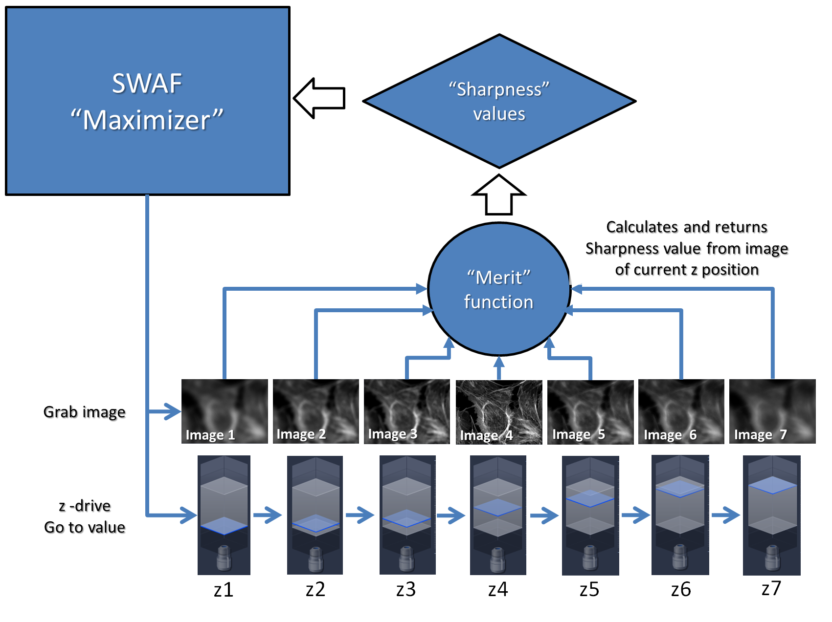
SWAF "Maximizer" linked to "Merit" function and "Sharpness" values diamond; arrows to Image 1-7 and z1-z7 — SWAF Workflow

The SWAF run is driven and controlled by the Maximizer which in turn controls the z-drive and camera to acquire a sequence of images at predefined axial intervals. Each of these images is transferred in sequence to a merit function that calculates a sharpness value for the image. This value is returned to the maximizer where a table of sharpness values is maintained. The Maximizer searches for (using either unidirectional (“full”) or bidirectional (“smart”) axial travel) and determines when a maximal sharpness value is found. Next data fitting is performed locally around the returned maximum to refine its position. Subsequently, the SWAF sets this z-value as the resulting axial position of the z-drive. If no maximum is found the Maximizer detects an error condition and throws a corresponding exception (error message). In this case the z-drive returns to its position of origin, thus minimizing the likelihood of a sample/ objective collision incident.

Software Autofocus Tool

Parameter		Description
Find Focus		Only visible in the tool on the Workflows tab. Starts an autofocus search to find the focus. The autofocus search is performed for the reference channel selected in the Channels tool.
Mode		Only visible if Show All is activated. Here you can select the sharpness measurement mode.
-	Auto	This is the default setting. If selected, the software makes a choice based on the configuration of the microscope. Such that for Widefield approaches or transmitted light the sharpness measure is always Contrast based. On the other hand, for optical sectioning methods (e.g. Spinning Disk) the software will automatically select an Intensity based approach to determine the sharpness values. If the microscope configuration cannot be detected automatically you can manually select the sharpness measurement mode.
-	Contrast	If selected the contrast-based mode will be used for sharpness measurement. This is the standard setting for Camera acquisition.
-	Intensity	If selected the intensity-based mode will be used for sharpness measurement. This is the standard setting for Confocal acquisition.
-	Reflex	Only available for LSM systems with imaging tracks other than MPLX and Airyscan SR. Using those tracks might lead to overexposure of the channel and failure for the Autofocus. If activated, the reflex of the laser on the cover glass surface is detected. An offset is used to focus onto the sample. You need to add the offset once by clicking the Find Offset button while the sample is in focus. The method requires a refractive index mismatch between the immersion medium and the cover glass and is therefore not for oil immersion objectives. For Reflex mode, the Search parameter should ideally be set to Smart. After the offset was defined, you can manually reduce the search range in order to facilitate shorter focusing times. The acquisition settings (e.g. laser line, PMT gain, emission filters) are configured automatically.
Quality		Only visible if Show All is activated. This parameter determines the merit function that will be used to calculate the contrast value of the image when Contrast mode is used by the SWAF (Software Autofocus) run to measure sharpness.
-	Default	If selected, a composite of weighted merit functions is used. Use this setting if the sample cover a greater part of the camera field of view.
-	Low Signal	If selected, a single merit function to determine the value is used. Use this setting if the image is noisy or the sample covers a small area of the field of view. As might be the case if you work with a calibration slide or beads.
Search		There are two options Smart and Full. These define a different type of primary maximizer used to run the SWAF, which in turn determines a number of additional characteristics and parameters of the entire process. To learn more about this, read the FAQ entry.
-	Smart	If selected, an alternative maximizer is used that can search in a bidirectional manner and will stop when a local maximum is found in the sharpness values (i.e. a significant decrease of sharpness in both z directions). Again if an error condition is detected the Smart maximizer will throw an exception. For specific information on the Software Autofocus using LSM Tracks in this context, also refer to chapter Software Autofocus Using LSM Tracks.
-	Full	If selected, the maximizer employed with this setting uses a unidirectional movement of the z-drive stepping through the entire relative or fixed search range defined in the SWAF tool (see Autofocus Search Range). The Full maximizer will return a global maximum for the autofocus run or throw an exception when an error condition is detected. For specific information on the Software Autofocus using LSM Tracks in this context, also refer to chapter Software Autofocus Using LSM Tracks.
-	Full No Checks	Searches the whole range and selects the sharpest level. Does not apply validity criteria to maximum.
Sampling		Here you can select the step size of how the search range is sampled.
-	Default	Uses the default step size (*dz = 1/sqrt(2) 2 * n* lambda/NA**).
-	Fine	Uses a small Z-distance (*0.5 dz**) between the individual focus images that are used to calculate the best focus position. This doubles the number of z-slices for the given range.
-	Medium	Uses a medium Z-distance (*2 dz**) between the individual focus images that are used to calculate the best focus position. Halves the number of z-slices for given range.
-	Coarse	Uses a large Z-distance (*4 dz**) between the individual focus images that are used to calculate the best focus position. Reduces number of z-slices by a factor of four.
Autofocus Search Range		Only visible if Show All is activated. Here you can switch between two distinct approaches for the autofocus search range:
-	Relative Range	This is the default mode. If selected, the software autofocus is calculated over a relative range.
-	Fixed Range	If selected, the software autofocus is calculated over a fixed range.
-	Automatic Range	Only visible if Relative Range is selected. Activated: Calculates the range for the autofocus search automatically depending on the objective set. Deactivated: Allows you to set the range manually with the Range input field.
-	Set Last	Only visible if Fixed Range is selected. Defines the current z-position as the end (last) point for the software autofocus. Alternatively, you can enter the desired value in the input field to the right of the button.
-	Range	Displays the area which is used for the autofocus search. If you have selected Relative Range, deactivate Automatic Range to adapt this parameter manually. If you have selected Fixed Range, you can adapt the range via the Set Last/Set First buttons or the input fields.
-	Step Size	Displays the selected Sampling distance between the individual focus images.
-	Set First	Only visible if Fixed Range is selected. Defines the current z-position as the start (first) point for the software autofocus. Alternatively, you can enter the desired value in the input field to the right of the button.
Autofocus ROI		Here you can define a spot meter or focus region such that the pixels evaluated by the SWAF are limited to a user defined region of the image. This is particularly usefully if you use a fiducial marker such as a speck of dirt or other constant artefact that serves as a reference for the sample focus at a fixed position over time. The autofocus ROI is displayed in the live image of the sample enabling it to be positioned and resized, as necessary. As an additional aid to help focusing you can also use the focus bar function of the live image that monitors the image contrast in the live image or spot meter ROI.
-	Spot Meter/Focus Region	Activated: Only uses the values from the Spot Meter/Focus Region to calculate the focus position. The Focus Region is displayed in the live image as a red dashed rectangle. You can adopt it by clicking on the frame and changing its size and position. Note that this option is not available for LSM acquisition.

Software Autofocus Using LSM Tracks

Confocal Tracks are also suitable as reference Channels for the Software Autofocus. As LSM acquisition is by design slower compared to Camera acquisition, some optimizations are done in the background in order to speed up the focusing action.

The typical measure for the correct focus position in confocal images is the intensity. Hence the aim of the SWAF is here not to generate images of a certain quality, but only to evaluate relative image intensities along the z-stack. This allows us to use very coarse scanning parameters.

Generally, the SWAF for LSM uses a fixed Frame Size of 64*64 pixels in combination with the fastest possible scan speed at the currently configured zoom. To further speed up the acquisition, bidirectional scanning is used. Whatever Laser power you specify in the Channels tool window for this Track is used during the SWAF action. Of note, while you assign a reference Channel, the corresponding Track with all its channels will be active during the focusing.

Some behavior depends on the selected Search Mode Full or Smart.

In the Full search, the system will use the detector gain as configured in the Channels tool window.

In contrast, the Smart search aims to start close to the likely intensity maximum of the z-Stack. This focus position is approximated by a fast line z-stack in the center of the image frame. As the line scan generates less pixels and a higher noise level, a useful dynamic range needs to be ensured. To this end, the fast line z-stack is repeated several times with increasing PMT gain. After the line scan, regardless if an intensity peak was found or not, a frame wise autofocus will follow.

In case no peak could be identified, e.g. because of a sparsely distributed sample, the Smart search will start at the original z-position and not optimization of the starting position will take place. Essentially, the Smart search will outperform the Full search on high Search Ranges and a highly varying effective focus position.