Colocalization View
Only visible for multichannel fluorescence images.
The channels that you are comparing with one another are displayed in the image area in the form of a color overlay. The channel color of the image is used here. If the images have more than 2 channels, you can add additional channels on the Dimensions tab. This temporary selection is deactivated, however, when you select the channels for comparison on the Coloc. Tools tab.
In the Colocal. (Colocalization) view, you can analyze the extent of colocalization quantitatively in two fluorescence channels. The view consists of two main areas: the X/Y scatter plot on the left and the actual image (2 channels are displayed) in the right image area. Using the Coloc. Tools tab, you can also display the colocalization table in the lower image area.
The analysis is performed on regions drawn into the image. Once a region is drawn, it is automatically treated as an active region. The scatter plot shows the pixel value frequencies for this region.
The Colocalization table displays the data for the entire image and for the selected region. To select several regions, press the Ctrl key while clicking on the desired regions.
Apart from drawing regions into the image, you can also draw them into the X/Y scatter plot. If you have used the function in the regions section of the Coloc. Tools tab, only those pixels that are framed by a region in the scatter plot are taken into consideration. This means that you can correlate interesting point clouds quickly with the corresponding pixels in the image.
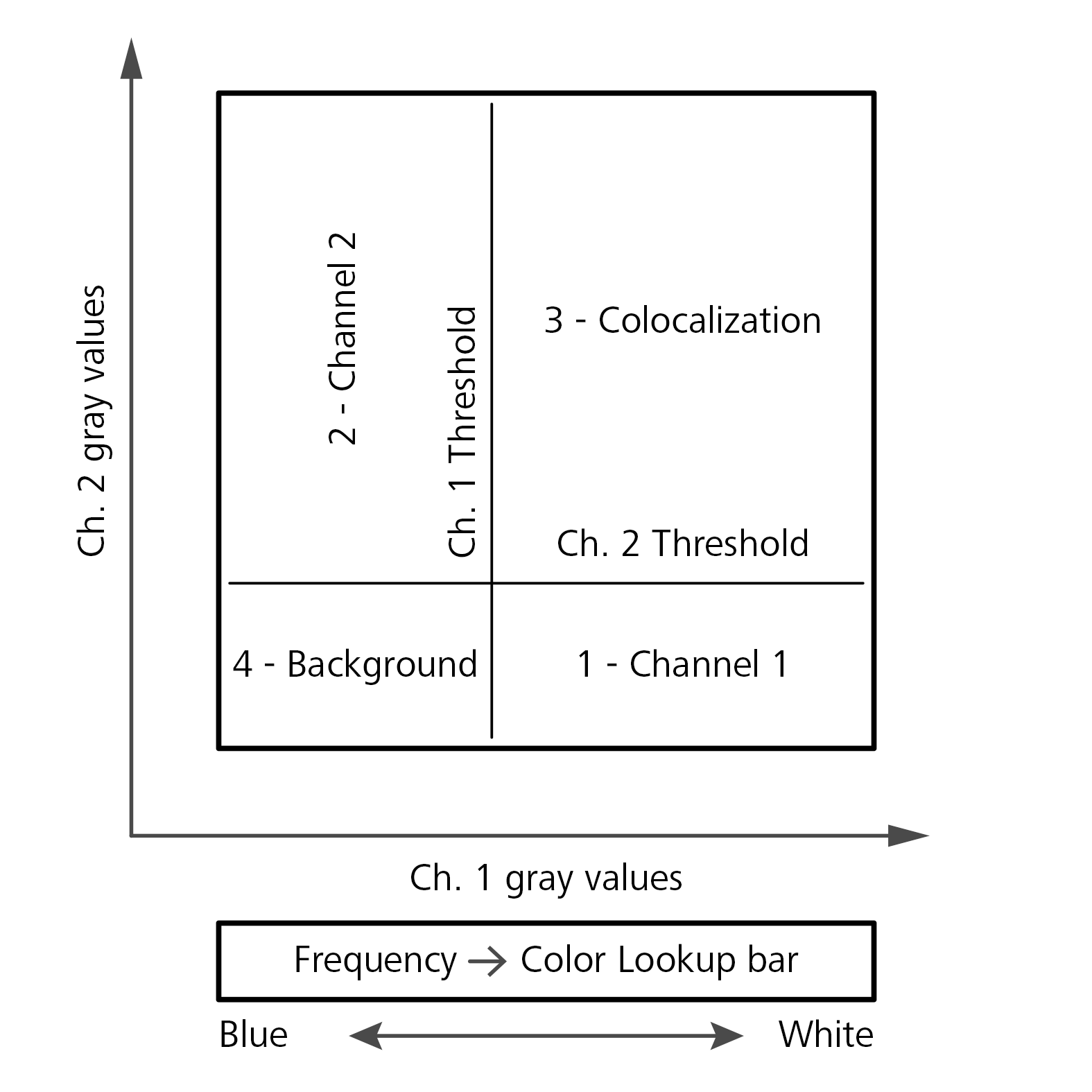
X/Y Scatter Plot
The pixel intensities of two channels are plotted against one another in the diagram and each pixel pair with the same X/Y image coordinates is displayed as a point. The frequency with which pixels of a certain brightness occur is visualized with a color palette that is displayed at the bottom of the diagram. The relative value range is between 0-255.
The vertical and horizontal axes show the gray value range of the relevant channel.
The diagram is overlaid with two lines that subdivide it into four quadrants, numbered from 1 to 4. Using the mouse, you can position the lines freely and adjust the threshold values to the data.
The quadrants have the following meanings:
- 1: Non-colocalizing pixels from channel 1
- 2: Non-colocalizing pixels from channel 2
- 3: Colocalizing pixels
- 4: Background
Coloc. Tools Tab
Here you find all control elements you need to perform a colocalization analysis.
|
Parameter |
Description |
|
|---|---|---|
|
Tool Bar |
Only visible if Show All is activated. Displays tools to draw regions for analysis into the image. For a description of the individual tools, see Graphics Tab. |
|
|
– |
ROI |
Only visible if you have drawn a region into the scatter plot. As long as this button is activated (highlighted in blue), you can select, move and change the regions in the scatter plot. If you want to change the quadrant lines again, you need to deselect the button. |
|
Channels |
Selects which channels of a multichannel image are compared with one another. Select a channel for both the horizontal and vertical diagram axis. The first and second channel are always selected by default. As soon as you have made a selection, all other channels are automatically removed from the image display. You can, however, add other channels temporarily on the Dimensions tab. |
|
|
Threshold |
Sets the threshold value (in gray levels) for both channels using the two Threshold sliders and the two spin boxes/input fields. |
|
|
Range |
Only visible if Show All is activated. Defines the grey value range displayed by the axes of the scatter diagram.. Auto is selected here by default, which means that the range is automatically set to the brightest pixel in the image. You can, however, enter a fixed gray value range between 256 (8 bits) and 65535 (16 bits). |
|
|
Dimension Selection |
Only visible if at least one of the Range dropdown lists is set to Auto and if the image is a z-stack or a time series. Defines whether the axis of the scatter plot is based on the values of the current image plane (2D), or on the entire z-stack (All Z)/time series (All T). In this way you can easily determine a valid diagram setting for an entire time series, for example, without having to analyze each individual time point. |
|
|
Costes |
Calculates the optimal threshold value according to Costes et al. |
|
|
Regions |
||
|
– |
Channel buttons |
Here you can mask pixels in the image according to which one of the four quadrants they belong to. The numbers on the buttons correspond to the numbering of the quadrants in the X/Y scatter plot. The color selection window is accessed by clicking on the color field. |
|
– |
Cut Mask |
Only active if a quadrant has been masked. |
|
– |
Opacity |
Only visible if Show All is activated. Define the degree of transparency of the masking. |
|
Extract |
||
|
– |
Scatter Plot |
Creates a new image document from the X/Y scatter plot. In the case of time series or z-stacks, the dimensions are also created automatically. |
|
– |
Table |
Only visible if Show All is activated. Creates a new table document. The document contains all measurement data from the colocalization analysis. All dimensions, such as T and Z, are also taken into account. This table can be saved as a *.csv document for further processing in other programs. |
|
– |
Table |
Only visible if Show All is activated. Activated: Displays the colocalization table in the image area. |