SEM Deconvolution

When a Scanning Electron Microscope (SEM) scans a sample, an electron beam is directed at a specific location. The scattered electrons are then captured by multiple detectors. Since the beam is not infinitely small, it illuminates not just a single point but an area, causing scattering from this entire region. Consequently, each pixel in the image contains information from an area around the corresponding point in the sample, rather than from a single point.

SEM Deconvolution is implemented as a regularized inverse filter with zero-order regularization. It uses a theoretical point spread function (PSF) to model the beam shape, which is then used to deblur the image and enhance high-frequency details in a robust manner. The regularized inverse filter aims to invert the influence of the beam profile on the image.

Point Spread Function (PSF) and Sigma Parameter

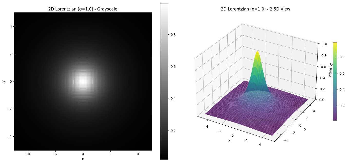
The PSF represents the distribution of the electron beam's intensity over the area it illuminates, and it is modeled as a 2D polar Lorentzian function in the following form:

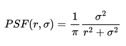
Here σ defines the Detail Enhancement and characterizes the width of this distribution, and r is the distance from any point in the image to the center. A larger σ indicates a wider beam, while a smaller σ corresponds to a more focused beam. Appropriate selection of σ is crucial for effective deconvolution.

Regularized Inverse Filter

This filter aims to reverse the effects of the blur introduced by the beam profile in the measurement. However, as inverting this effect is an ill-posed problem, regularization is necessary due to:

• Stability: It helps in stabilizing the inverse filter, making it less sensitive to noise and numerical errors.
• Noise reduction: It prevents the amplification of noise, which is common when directly applying an inverse filter.
• Robustness: The regularized solution is more robust to variations in the data and model inaccuracies.

Zero-order regularization refers to regularization based on an accelerated G-difference method modeled on Tikhonov.

Reference: Schaefer LH, Schuster D, Herz H. Generalized approach for accelerated maximum likelihood based image restoration applied to three-dimensional fluorescence microscopy. J Microsc. 2001 Nov;204(Pt 2):99-107. doi: 10.1046/j.1365-2818.2001.00949.x. PMID: 11737543.

Optimal Setting of the Smoothing and Detail Enhancement Parameters

To optimally set the smoothing and detail enhancement values, you should consider the characteristics of your acquisition, for example:

• Beam width: Knowledge of the beam width can guide the selection of Smoothing parameter for the PSF.
• Noise level: Higher noise levels may require stronger regularization (Detail Enhancement) to prevent noise amplification.
• Desired sharpness: You can adjust the Detail Enhancement strength to balance between noise reduction and sharpness.

See also

• SEM Deconvolution Tool

This tool enables you to execute a deconvolution on your SEM data. For a detailed description of the process and algorithm, see Process and Algorithm of SEM Deconvolution.