Cast Iron Analysis
This module enables you to analyze the size (1-8), shape (I-IV) and distribution (A-E) of graphite particles in cast iron samples in accordance with DIN EN ISO 945 - 2019. Additionally, you can investigate the nodularity, calculate the spherodial number (including shape class IV) and analyze the area percentage of the graphite particles in the image. According to the standard, two options (by Number or by Area) for the calculation of the statistical results are available.
See also
The Concept
The operating concept of the Cast Iron Analysis module is designed to make it possible to achieve a reproducible result with as little interaction as possible. The performance of a measurement can be automated to such an extent that only the project data need to be entered and the entire analysis process can run automatically.
To automate a measurement completely, you need extensive knowledge of systems engineering and the respective application. Carelessly made alterations of a setting can promptly lead to faulty measurement results. It is important, therefore, to prevent users not having such knowledge from changing the basic settings. This is achieved by dividing up the tasks involved into the definition of an analysis and the performance of an analysis. For this reason, the operation of the module sticks to the general operating concept of the software:
- Creating and Managing Jobs (Supervisor)
- Create job templates for cast iron analysis, manage templates, view job results, sign & release jobs (with GxP module only). Note that under Job Mode you will find a sample workflow within a pre-defined job template for cast iron analysis.
- Running Jobs (Operator)
Performing cast iron analysis using pre-defined job templates.
See also
General Preparations
A pre-defined job template is included in the software, when you have licenced the Cast Iron Analysis module. You can modify the job template, see Working with Job Templates.
As a Supervisor you can access/edit the job template under Manage Templates. On the left side in the Categories list under Material Modules select Cast Iron Analysis.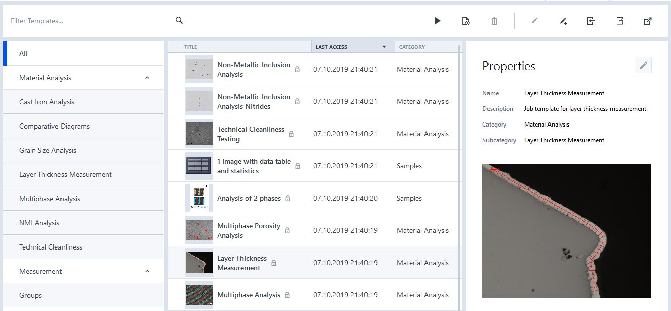
In the templates list you see the available job template. Select the entry, and from the context menu, open the job template. The job templates generally contains three major tasks:
|
1 |
Filling out an Input Form |
|
2 |
Performing the Analysis |
|
3 |
Creating a Report |
General Analysis Workflow
The analysis steps of the workflow contains the following substeps to be executed. In this example the substeps are created within a Loop Task (1), meaning all included steps will be repeated depending on the loop settings. Regarding this you can easily fulfill the normative requirements of repeating the identical steps of an analysis for several times.
Note that greyed out task icons are set to "Run silent". The tasks will not be shown when the workflow is executed. To activate them, right-click on the icon and deactivate the Run silent menu entry.
|
Workflow Step |
Description |
|
|---|---|---|
|
Loading an Image (2) |
Load your image you wish to analyze. The workflow can be adapted to perform image acquisition tasks here as well. |
|
|
Validating the input image (2) |
This task is recommended to use right after loading or acquiring an image. Currently it will check if the input image has the correct scaling information. This is important to make sure the image can be processed correctly. |
|
|
Processing the Image (2) |
Perform improvements on the image, e.g. change Brightness, Contrast and/or Gamma. |
|
|
Performing the Analysis (3) including: |
This step is the heart of each method. Each analysis can be stored as Analysis Settings File. Depending on the selected method the software will provide the specific parameters. Each method is described in detail in the following chapters. |
|
|
- |
Setting Up the Classes |
For the sample workflow all necessary classes are pre-defined. This step is set to run silent because of that. |
|
- |
Setting Up the Measurement Frame/Pattern |
Adjust the region/area which has to be analyzed. |
|
- |
Segmenting the Image |
Segment the image automatically by clicking inside the image. |
|
- |
Interactively Adjust the Segmentation Results |
Edit the segmentation result interactively. |
|
- |
Setting up the features |
Apply specific measurement features to the image. |
|
- |
Viewing the Measurement Data |
The segmented image and tables including measurement results are displayed. |
|
- |
Determining the Graphite Distribution |
This step is another interactive step. You have to manually determine the graphite distribution by comparing the acquired image with the images from the standard. The results have to be entered in the Graphite Distribution Setup tool. |
|
Showing the Results View (4) |
The Results View is displayed containing the analysis results and statistics. |
|


Cast Iron Analysis
This topic explains the specific image analysis part of the Cast Iron Analysis job template which is delivered with the software. We recommend that you read the sections General Preparations and General Analysis Workflow to make yourself familiar with the general workflow.
Frame Setup
Setting up a frame for the cast iron analysis is an optional step. If you want to, you can add a specific measurement frame (e.g. rectangle area in the center of the sample) which then will be used for the analysis only. Whether you want to use a measurement frame is depending on your sample and individual processes. The tool offers everything you need to setup the frame properly. By using the tool parameters you can adjust the frame individually. The value Inside Only in the Mode field is required by the standard. For this reason, it is not editable.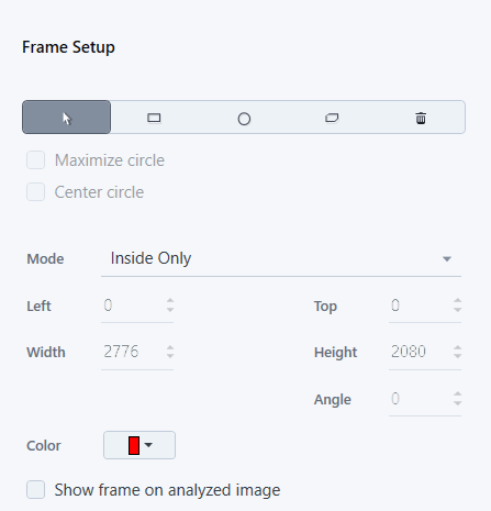
Image Segmentation Setup
In this step the software segments the individual graphite particles of the cast iron sample. To start the segmentation, click on a graphite particle within the image. The software then displays the results according to the specified overlay colors for the different classes. Repeat the segmentation by clicking on not detected particles in the image, in case some areas have not been detected correctly.
To change the display of the segmentation (size instead of shape), activate Graphite Particle Size in the Image Analysis Options tab below the image area. The tool offers all parameters which are necessary to optimize the segmentation result.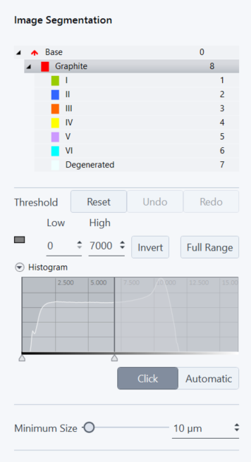
A minimum size of 10 µm (Feret max. diameter) is recommended by the standard DIN EN ISO 945.
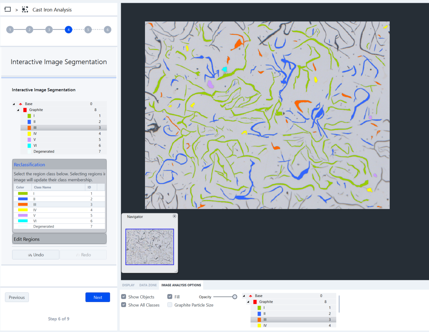
Interactive Image Segmentation Setup
In this step you can adjust the segmentation result interactively. In the Reclassification tool you can correct wrong classified particles. Select the correct class from the list and click on the wrongly classified particle within the image. The particle will be reclassified with the selected class. You can also mark degenerated graphite by selecting the class Degenerated and then click on the degenerated particles in the image. To edit the segmentation results use the tools under Edit Regions.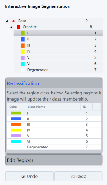
Graphite Distribution Setup
This is an optional step. Here, you have to manually determine the graphite distribution by comparing the acquired and segmented image with the images from the standard. Enter the results in the corresponding input fields.
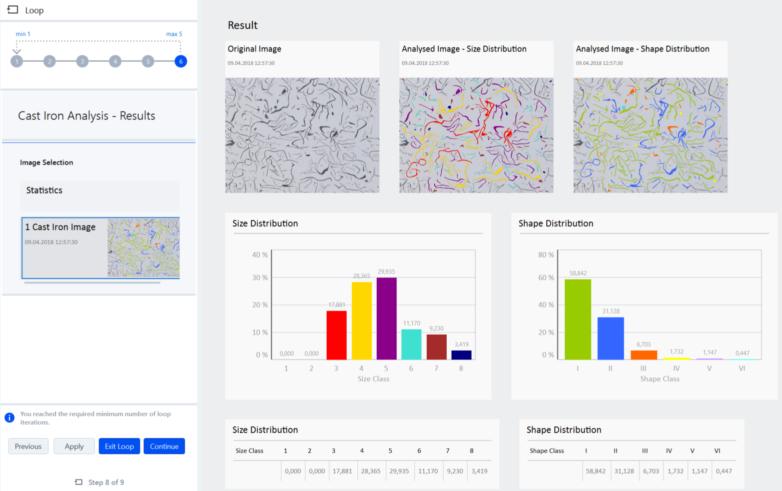
Result View
At the end of each analysis the Result view is displayed. It shows all images and results of the analysis which was performed. Additionally, the original images are displayed as well. In the Image Selection tool on the left side you can exclude images you do not want to have displayed within the result. If you click on the Statistics section within the tool, you can display all results of the analysis in a clearly structured table view.
Additional Results
|
Parameter |
Description |
|---|---|
|
Nodularity |
The calculation of the nodularity depends on the selected statistic in the Form template. Activated: Statistic by number Nodularity = (NVI + NV) / (Nall) * 100% -> % Nodularity Activated: Statistic by area (default) Nodularity = (AVI + AV) / (Aall) * 100% -> % Nodularity The default value is recommended by Standard DIN EN 945-4:2019. |
|
Spheroidal number & Nodule count |
The formula for the spheroidal number (according ISO 945-1) is as follows: Spheroidal number = (NVI + NV) / Area -> number of nodules (shape class V and VI + optional IV) |
|
Graphite Content % |
Area fraction of graphite particles based on the measuring area. It will be calculated as follows: A (particles) / A (summation) Particles are cut at the measurement frame or image frame even though inside only is set for the frame by default. |
|
Graphite particle count |
Total number of graphite particles (segmented phases) divided by the test area in mm². |